Chapter 2: exponential families and mixture families

Chapter 2 · book pp. 31–50 · Shun-ichi Amari, Information Geometry and Its Applications (2016)

exponential-familycumulant-generating-functiongaussiannatural-parameter

Notes for Chapter 2 of Amari, Information Geometry and Its Applications (Springer, 2016), DOI 10.1007/978-4-431-55978-8. No text of the book is reproduced here. The next section summarises the book’s chapter in my own words, in the book’s order. The sections after it are explorations that I asked for, one at a time, so they follow my questions and not the book’s order.

Previous chapter: Chapter 1: the dually flat structure.

What the chapter covers (a summary of the book’s chapter)

The chapter studies the exponential family of probability distributions. It contains many familiar families (discrete distributions, Gaussians, multinomials, gammas), and it comes with a convex function, the cumulant generating function (the “free energy” of physics). Applying Chapter 1 to that function gives a dually flat structure whose divergence is the KL divergence, whose metric is the Fisher information, and whose two affine coordinate systems are the natural parameters and the expectation parameters of statistics. The mixture family is its dual. The chapter ends with applications of the Pythagorean theorem. The sections in order:

§2.1 The exponential family. The standard form is p(x;\theta)=\exp\{\theta\cdot x-\psi(\theta)\} with respect to a base measure, where the statistics x_i=h_i(x) must be linearly independent. The normalisation defines \psi(\theta)=\log\int e^{\theta\cdot x}d\mu, which is convex by Chapter 1. The natural parameter \theta is one affine coordinate system. Its dual, from the Legendre transformation, is the expectation parameter \eta=\nabla\psi(\theta)=\mathbb E[x], and the dual potential \varphi(\eta) is the negative entropy. The Bregman divergence of \psi turns out to be the KL divergence with its arguments reversed, and the metric \partial_i\partial_j\psi is the Fisher information (Theorem 2.1).
§2.2 Two examples. The Gaussian, with statistics (x,x^2), natural parameters (\mu/\sigma^2,\,-1/(2\sigma^2)) and expectation parameters (\mu,\,\mu^2+\sigma^2). The discrete distributions on \{0,\dots,n\}, with the indicator functions as statistics, the log-odds against outcome 0 as natural parameters, \psi=\log(1+\sum e^{\theta_i}), and the probabilities themselves as expectation parameters.
§2.3 The mixture family. A family p=\sum\eta_iq_i(x) of mixtures of fixed distributions. The discrete simplex is both an exponential and a mixture family. For a general mixture family the negative entropy is still convex in \eta, so it also has a dually flat structure, but its other coordinates are not the natural parameters of an exponential family.
§2.4 e-flat and m-flat. A straight line in \theta is an e-geodesic: it interpolates the logarithms of the two densities and is itself a one-dimensional exponential family. A straight line in \eta is an m-geodesic: it interpolates the expectations, which for discrete distributions is the ordinary mixture. Submanifolds defined by linear constraints in \theta are e-flat, and in \eta are m-flat.
§2.5 The infinite-dimensional manifold. The space of all densities is treated, in a naive way, as an exponential and a mixture family at once, using delta functions as the generating distributions: \theta(s)=\log p(s)+\psi and \eta(s)=p(s). The e- and m-geodesics, the KL divergence, the Pythagorean theorem and the Fisher metric all carry over formally. The book warns that this is not mathematically justified: KL neighbourhoods fail to define a topology and the entropy is not continuous there.
§2.6 The kernel exponential family. A model with a function \theta(y) as natural parameter, built from a positive-definite kernel k(x,y), with dual parameter \eta(y)=\mathbb E[k(x,y)]. It does not cover all densities, and §2.5 is the special case of a delta-function kernel.
§2.7 Bregman divergences and exponential families. The converse of §2.1: given a Bregman divergence one can build an exponential family whose KL divergence it is (finding the base measure is an inverse Laplace transform). Theorem 2.2: regular exponential families and regular Bregman divergences are in one-to-one correspondence. A mixture family is dually flat but is not thereby an exponential family.
§2.8 Applications of the Pythagorean theorem. (§2.8.1) Maximum entropy: among all distributions with prescribed averages, the max-entropy one is the e-projection of the uniform distribution onto an m-flat sheet, and the family of such answers is an exponential family. (§2.8.2) Mutual information: the independent distributions form an e-flat family, the m-projection of a joint distribution onto it is the product of its marginals, and the KL divergence to the product is the mutual information. (§2.8.3) Repeated observations and maximum likelihood: with N independent observations, the potential, the KL divergence and the metric are multiplied by N and the dual affine structure is unchanged; the maximum likelihood estimator in a submodel is the m-projection of the observed point (the histogram) onto it.
Closing remarks. Exponential families are the natural setting for studying dual flatness and statistical inference, and every discrete model sits inside one. For continuous variables many models are only curved subfamilies of exponential families, and non-exponential models can be approximated locally by a larger exponential family.

A Gaussian family and its cumulant generating function

The chapter’s opening line says that an exponential family is associated with a convex function, the cumulant generating function \psi (the “free energy”). Two pictures show what that means for Gaussians.

One parameter: only the mean moves. Fix the width and slide the mean. Each member of the family is a bell curve, and each is one point on the curve of \psi.

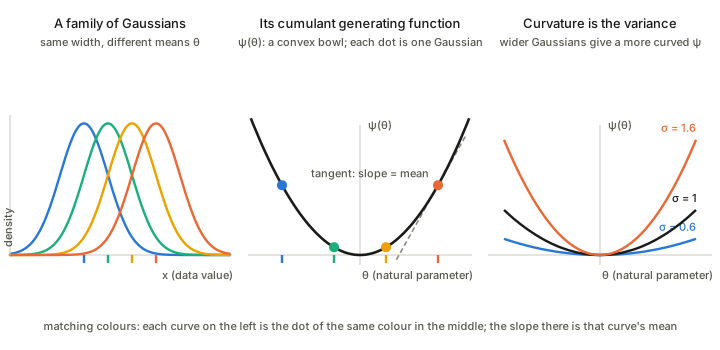
Left: four bell curves of equal width with different means. Middle: a convex bowl, psi of theta, with four coloured dots matching the four bell curves and a dashed tangent line at one of them. Right: the same bowl for three different widths; a wider Gaussian gives a more sharply curved bowl. — Left: a one-parameter Gaussian family. Middle: its cumulant generating function \psi(\theta); each dot is the bell curve of the same colour, and the slope at a dot is that curve’s mean. Right: the same function for three widths: the wider the Gaussian, the more curved the bowl.

The function does the bookkeeping for the whole family. Its slope at a point is the mean of the distribution there, and its curvature is the variance. So a single convex function holds both the average and the spread of every member, and this is the reason the Hessian of \psi is the Fisher information (the Fisher information).

Where \psi comes from, for the one-parameter family. Fix the width \sigma and start from one reference density, the zero-mean Gaussian h(x)=\frac{1}{\sqrt{2\pi\sigma^2}}e^{-x^2/(2\sigma^2)}. The family is a tilt of h by e^{\theta x}, renormalised:

p(x;\theta)=h(x)\,e^{\theta x-\psi(\theta)} .

Step 1: normalisation defines \psi. The tilted function h\,e^{\theta x} is generally not a probability density, so we divide it by a constant that depends on \theta but not on x; writing that constant as e^{\psi(\theta)} is just naming the normaliser on a log scale. Requiring \int p\,dx=1 and pulling the x-independent factor e^{-\psi(\theta)} out of the integral gives e^{\psi(\theta)}=\int h(x)\,e^{\theta x}dx, that is

\psi(\theta)=\log\mathbb E_h\!\left[e^{\theta x}\right].

This is the log of the moment generating function of h, hence the name cumulant generating function (in physics, the log of the partition function, the “free energy”). Nothing here is Gaussian yet: the form h\,e^{\theta x-\psi} is the definition of an exponential family, and \psi is forced by normalisation.

Step 2: complete the square. The Gaussian enters only through h. Combine the exponents: \theta x-\frac{x^2}{2\sigma^2}=-\frac{(x-\sigma^2\theta)^2}{2\sigma^2}+\frac{\sigma^2\theta^2}{2}. So \int h\,e^{\theta x}dx=e^{\sigma^2\theta^2/2}\times\big(\text{a full Gaussian density with mean }\sigma^2\theta\big), and the density integrates to 1.

Step 3: the answer.

\psi(\theta)=\tfrac12\,\sigma^2\theta^2 .

For unit width this is the parabola \theta^2/2 in the middle panel of the figure. Reading it back:

The members are Gaussians. Tilting a zero-mean Gaussian by e^{\theta x} only shifts it: p(x;\theta)=\mathcal N(\sigma^2\theta,\ \sigma^2).
Slope is the mean: \psi'(\theta)=\sigma^2\theta=\mu, so \theta=\mu/\sigma^2, the first natural parameter of the full family below.
Curvature is the variance: \psi''(\theta)=\sigma^2, a constant, so the Fisher information is the same everywhere along this family, and wider Gaussians give a more curved bowl (right panel).
Why the bowl is an exact parabola. The Taylor coefficients of a cumulant generating function are the cumulants. A Gaussian has only a mean and a variance, and every higher cumulant vanishes, so the series stops at the quadratic term. A non-Gaussian family has higher-order terms and a bowl that is not exactly a parabola.

Two parameters: the full Gaussian family. Let the mean and the width both vary. The natural parameters are \theta_1=\mu/\sigma^2 and \theta_2=-1/(2\sigma^2), so the allowed region is only the half-plane \theta_2<0.

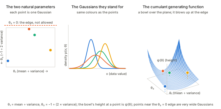
Left: the plane of the two natural parameters with a forbidden edge at the top and four coloured points. Middle: the four Gaussians that the points stand for. Right: the cumulant generating function drawn as a bowl over the parameter plane, rising steeply toward the forbidden edge, with the four coloured points on the bowl. — Left: the parameter plane; each point is one Gaussian, and the edge \theta_2=0 is not allowed. Middle: the Gaussians those points stand for. Right: the cumulant generating function as a bowl over the plane; each Gaussian is a coloured point on it.

Three things to see. First, the function is a bowl over a half-plane, not the whole plane: the parameters are only meaningful while the variance is positive. Second, the bowl climbs without limit as a point approaches the forbidden edge, which is where the Gaussian becomes infinitely wide. Third, the same recipe works as before: the slope of the bowl (now a two-component gradient) gives the expectation parameters (\mu,\ \mu^2+\sigma^2), and its curvature (now a matrix) gives the covariance of (x,x^2), the Fisher matrix.

A kernel exponential family, the simplest case

An ordinary exponential family multiplies a few fixed functions of x (such as x and x^2) by weights \theta_i, adds them up in the exponent and normalises. The book’s kernel exponential family (§2.6, due to Fukumizu) does the same with bumps k(x,y), one around every point y, and a whole function \theta(y) of weights, one for each point y:

p(x;\theta)=\exp\Big\{\int\theta(y)\,k(x,y)\,dy-\psi[\theta]\Big\}\quad\text{with respect to a base measure }d\mu(x).

Here k is a positive-definite kernel (see the kernel functions page for what that means), for example the Gaussian kernel k_\sigma(x,y)\propto e^{-(x-y)^2/(2\sigma^2)} with width \sigma, and the base measure is a suitable fixed one, for instance d\mu(x)=e^{-x^2/(2\tau^2)}dx. The natural parameter is the function \theta(y) (instead of a list \theta_i), the dual parameter is the function \eta(y)=\mathbb E[k(x,y)], the average of the bump at y, and \psi[\theta] is a convex functional of \theta. The book stresses that this family does not cover every density: there are many such models, one for each choice of k and d\mu. The “naive treatment” of the space of all densities in §2.5 is the special case where the kernel is a delta function, k(x,y)=\delta(x-y).

The simplest picture: two centres. Replace the continuum of points y by just two centres c_1,c_2, so the weight function is concentrated on them, \theta(y)=\theta_1\delta(y-c_1)+\theta_2\delta(y-c_2). The integral becomes a sum and the family is

p(x;\theta)\;\propto\;\exp\{\theta_1k(x,c_1)+\theta_2k(x,c_2)\}\quad(\text{times the base measure}),

an ordinary two-parameter exponential family whose two “statistics” are the two bumps. The figure draws it with a uniform base measure on a fixed interval, to keep it simple; the book’s example base measure is the Gaussian-weighted one above.

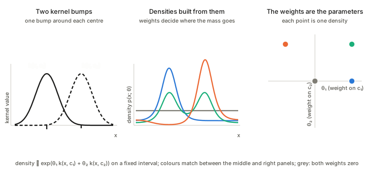
Left: two bump-shaped kernels, one solid and one dashed, centred at two points on a line. Middle: four densities built by weighting the two bumps and exponentiating: a flat grey one for zero weights, a blue one with a peak at the left centre, a green one with a peak at each centre, and an orange one with a tall peak at the right centre and a dip at the left. Right: the plane of the two weights, with four coloured points that are the four densities. — Left: two kernel bumps. Middle: densities built from them; each curve is one choice of weights. Right: the two weights are the parameters, and each coloured point is the density of the same colour in the middle panel.

Read the picture from left to right. The two bumps are fixed once and for all. A choice of the two weights, one point in the right panel, gives one density in the middle panel. Zero weights give the flat grey density. A positive weight on a bump piles probability near its centre (blue, left bump), positive weights on both give two peaks (green), and a negative weight on one bump pushes probability away from its centre (orange has a dip at the left centre). So the weights are the natural parameters, the dual parameters are the averages \eta_i=\mathbb E[k(x,c_i)] of the two bumps, and everything said about exponential families applies: \psi is convex, its slope gives the averages of the bumps and its curvature gives how they co-vary. With many centres the same construction becomes the function-valued \theta(y) of the book.

From two centres to a whole function \theta(y)

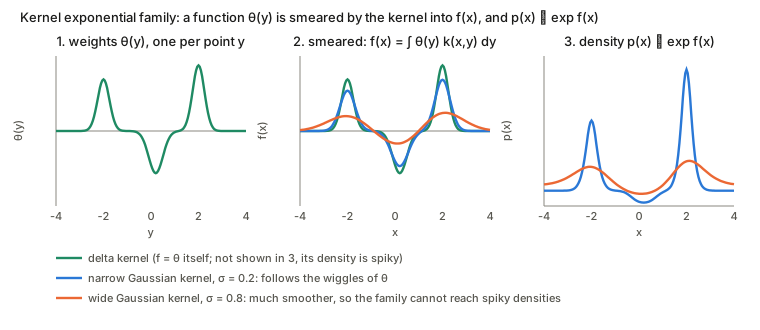
The two-centre family has two weights. The kernel exponential family lets every point y carry a weight, so the parameter is a function \theta(y). The only new idea is the middle step: the weights are not used directly, they are smeared by the kernel into a function of x,

f(x)=\int\theta(y)\,k(x,y)\,dy,\qquad p(x)\;\propto\;e^{f(x)}\ \ (\text{times the base measure}).

So f is the log-density up to a constant, and it is always a blurred copy of \theta. The kernel decides how much blurring: a Gaussian kernel of width \sigma averages \theta over a window of that width.

Left: a weight function theta of y with two positive bumps near minus 2 and plus 2 and a negative dip near 0. Middle: the smeared function f of x for a delta kernel (same as theta), a narrow Gaussian kernel (nearly the same, slightly rounded) and a wide Gaussian kernel (much flatter bumps and dip). Right: the densities made by exponentiating f, sharply peaked for the narrow kernel and gentle for the wide kernel. — Left: one choice of the weight function \theta(y). Middle: the same \theta smeared by three kernels. Right: the densities p\propto e^{f} for the two Gaussian kernels. Positive weight piles probability up and negative weight digs a dip, as with the two bumps, but the kernel width limits how sharp the result can be.

What the figure shows:

A delta kernel does no smearing, so f=\theta and the log-density can be any function. This is the “naive” space of all densities of §2.5.
A narrow kernel blurs only a little, so f still follows the wiggles of \theta and the family can reach sharp-looking densities.
A wide kernel blurs a lot. Whatever \theta you choose, f comes out smooth, so the family contains only smooth densities. This is the sense in which the family does not cover every density, and why each choice of k is a different model.
The dual parameter has the same picture in the other direction: \eta(y)=\mathbb E[k(x,y)] is the density p itself smeared by the kernel, a function of y.
Why the kernel must be positive definite: so that a nonzero \theta cannot be smeared into nothing, which keeps \psi[\theta] convex and the dual pair of coordinates well defined.

The maximum entropy principle (§2.8.1)

The question. You do not know a distribution on the outcomes, but you do know the average of some quantities of the outcome, for instance the average face value of a die. Many distributions agree with what you know. Which one should you pick? The maximum entropy principle says: with nothing else to go on, pick the one with the largest entropy, the one that assumes the least beyond what you know.

In the book’s notation there are k functions c_1(x),\dots,c_k(x) of the outcome, and the known averages are \mathbb E[c_i(x)]=a_i.

Left: the triangle of distributions on three outcomes with the uniform distribution P0 at the centre and grey contour lines of equal entropy around it. A straight orange line M(a) is the sheet of distributions with a prescribed average. It touches one entropy contour at the point P-hat, which lies on a blue curve running from the uniform distribution, the family of maximum-entropy points. Another distribution P is marked on the orange line. Right: the entropy along the orange line, rising to one peak at P-hat, with P lower on the curve. — Left: all distributions on three outcomes. The orange line holds those that satisfy the prescribed average; the grey contours are lines of equal entropy around the uniform distribution P_0. The orange line touches the highest reachable contour at \hat P. Right: along the orange line the entropy has one peak, at \hat P.

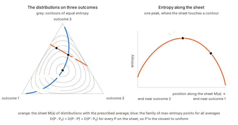
Step 1: the constraints cut out a flat sheet. All distributions with the prescribed averages form a sheet M(a) inside the set of all distributions, of dimension n-k when there are n+1 outcomes and k constraints. It is m-flat (straight in the probabilities, the orange line in the picture), because a mixture of two distributions that both have the prescribed averages has them too.

Step 2: entropy is a distance to the uniform distribution. The uniform distribution P_0 has the largest entropy of all, and its natural parameters are zero, \theta_0=0. The book shows that the divergence D_{\mathrm{KL}}[P:P_0] is the negative entropy of P plus a constant. So maximising entropy is the same as getting as close as possible to the uniform distribution in KL divergence: in the picture, reaching the highest entropy contour that the sheet can touch.

Step 3: Pythagoras picks the point. Let \hat P be the point of M(a) with the largest entropy. For every other P in the sheet,

D_{\mathrm{KL}}[P:P_0]=D_{\mathrm{KL}}[P:\hat P]+D_{\mathrm{KL}}[\hat P:P_0].

This is the generalised Pythagorean theorem of Chapter 1. The second term is the same for every P, and the first is positive unless P=\hat P, so \hat P is the closest point to the uniform distribution. Geometrically, \hat P is the e-projection of P_0 onto M(a): the e-geodesic from P_0 to \hat P meets the m-flat sheet at a right angle.

Step 4: the answer is an exponential family. Change the prescribed averages and the sheet moves, and so does its maximum-entropy point. All these points \hat P(a) together form a k-dimensional family, the blue curve, and it is an exponential family:

\hat p(x;\theta)=\exp\{\theta\cdot c(x)-\psi(\theta)\}.

In words: the maximum-entropy distribution for given averages is the uniform distribution tilted by an exponential of the quantities you constrained. The tilts \theta are the Lagrange multipliers of the constraints. The book’s variational derivation (maximising entropy under the constraints) gives the same result.

How the maximum entropy principle follows from the Pythagorean theorem

Step 3 above used the theorem in one line. Spelled out, it is three links, and the picture shows all of them.

Left: a sketch of a right-angled triangle. The uniform distribution P0 is joined by a blue curve, the e-geodesic, to the point P-hat on an orange line, the sheet of allowed distributions, meeting it at a right angle. Another allowed distribution P lies further along the sheet; the legs are labelled D of P-hat from P0 and D of P from P-hat, and the hypotenuse D of P from P0. Right: the divergence from the uniform distribution along the sheet is a bowl. A blue band up to its lowest level is D of P-hat from P0, the same for every P, and the orange region above that level is D of P from P-hat; the bowl bottoms out at P-hat. — Left: the right triangle P_0,\hat P,P. The right angle is measured in the Fisher metric, so it does not look like a right angle in every chart. Right: the distance from the uniform distribution along the sheet. Its lowest level is the fixed piece D(\hat P:P_0) and what sits above that level is D(P:\hat P).

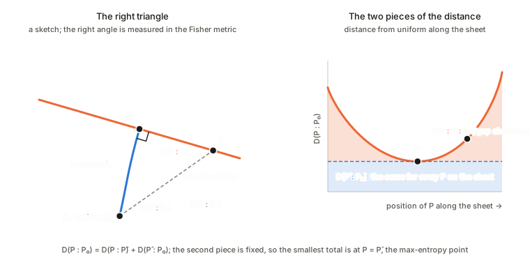
Entropy is a distance to the uniform distribution. When P_0 is uniform, D_{\mathrm{KL}}[P:P_0] equals a constant minus the entropy of P. So maximising entropy is the same as minimising D_{\mathrm{KL}}[P:P_0].
The constraint set is m-flat. The distributions with the prescribed averages form the sheet M(a), straight in the expectation parameters \eta. Let \hat P be its max-entropy point.
The e-geodesic from P_0 to \hat P meets the sheet at a right angle. The point \hat P is the exponential tilt of P_0 by the constrained functions c(x), so the e-geodesic leaves P_0 in the direction c. A tangent direction of the sheet leaves every \mathbb E[c_i] unchanged, and that is exactly the vanishing of the pairing between the two directions in the Pythagorean theorem.

Then, for every other P on the sheet, D(P:P_0)=D(P:\hat P)+D(\hat P:P_0). The second piece is the same for every P (the blue band in the right panel), and the first is never negative (the orange region), so the smallest total is at P=\hat P. Since entropy is a constant minus D(P:P_0), that point has the largest entropy. The Gibbs-inequality argument in the derivation below is this same identity read the other way round: the entropy gap between P and \hat P is the divergence D_{\mathrm{KL}}[P:\hat P].

A concrete example: a die with average 4.5

You have a six-sided die and the only thing you know is that its long-run average roll is 4.5, not the fair 3.5. Which probabilities should you assign to the faces? Many distributions fit: all the probability on faces 3 and 6 in equal parts, or a spike on face 6 over a flat floor, and so on. The maximum entropy principle picks the one that assumes the least beyond “the average is 4.5”.

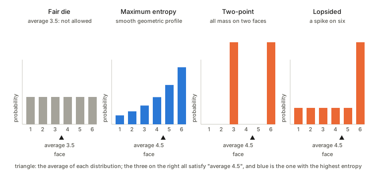
Four bar charts of probabilities for the six faces of a die. The fair die with average 3.5 is flat and does not satisfy the constraint. The maximum entropy distribution with average 4.5 rises smoothly and geometrically from face 1 to face 6. A two-point distribution has all its probability on faces 3 and 6. A lopsided one is flat on faces 1 to 5 with a spike on face 6. A small triangle under each chart marks its average. — The fair die (grey) is not allowed, because its average is 3.5. The three distributions on the right all have average 4.5. The maximum entropy one (blue) is the smooth geometric profile, the others are lumpy.

In the notation above the outcomes are the six faces, the constraint function is the face value c(x)=x, the prescribed average is a=4.5, the sheet M(a) is the set of all distributions with that average, and the centre P_0 is the fair die.

The answer is the uniform distribution tilted by e^{\theta x}. The maximum entropy distribution is \hat p(x)\propto e^{\theta x} for x=1,\dots,6: each face is a fixed multiple of the one before, so the probabilities rise geometrically. Only \theta has to be found, so that the average comes out right; it is about 0.37, which makes each face roughly 1.45 times as likely as the previous one.
The other candidates have less entropy. The two-point and the lopsided distributions both satisfy the constraint, but each puts probability in lumps, and each has lower entropy than the geometric profile. The fair die has the largest entropy of all, but it is not on the sheet.
Pythagoras holds. For any other distribution P with average 4.5, D_{\mathrm{KL}}[P:P_0]=D_{\mathrm{KL}}[P:\hat P]+D_{\mathrm{KL}}[\hat P:P_0], so no distribution on the sheet is closer to the fair die than \hat P.
\theta is a multiplier. It is the Lagrange multiplier of the constraint “average =4.5”: the price, in log-probability, of one extra point of face value. Move the average back to 3.5 and \theta=0, the fair die. Move it toward 6 and the geometric profile steepens and piles more and more mass on face 6. A constraint on the variance too would add x^2 to the exponent.

Deriving the maximum entropy die

The geometric shape is not a guess: it is forced by the constraint. Choose p_1,\dots,p_6 to maximise the entropy H(p)=-\sum_x p_x\log p_x subject to \sum_xp_x=1 and \sum_x x\,p_x=4.5.

Step 1: Lagrange multipliers. Fold the constraints into one function, with a multiplier for each,

L=-\sum_{y}p_y\log p_y-\lambda_0\Big(\sum_yp_y-1\Big)-\lambda_1\Big(\sum_yy\,p_y-4.5\Big),

and require the derivative with respect to every p_x to vanish. (The summation index is called y so that x can mean the one face being differentiated.) Every sum has one term per face, and \partial/\partial p_x only touches the term with y=x, so all the other terms differentiate to zero:

the entropy term: by the product rule, \frac{\partial}{\partial p_x}(p_x\log p_x)=\log p_x+p_x\cdot\frac1{p_x}=\log p_x+1, so the term contributes -\log p_x-1;
the normalisation term: p_x appears once with coefficient 1, so it contributes -\lambda_0;
the mean term: p_x appears as x\,p_x, where the face value x is a constant, so it contributes -\lambda_1x.

Together,

\frac{\partial L}{\partial p_x}=-\log p_x-1-\lambda_0-\lambda_1x=0 .

The surprising “-1” comes from the product rule on p\log p; it does not matter in the end, because it is absorbed into the normaliser.

Step 2: read off the shape. Solving for p_x gives p_x=e^{-1-\lambda_0}\,e^{-\lambda_1x}. The first factor does not depend on x, so write \theta=-\lambda_1 and call that constant 1/Z:

p_x=\frac{e^{\theta x}}{Z},\qquad Z=\sum_{x=1}^6e^{\theta x}.

The ratio of neighbouring faces is p_{x+1}/p_x=e^{\theta} for every x: each face is the same multiple of the previous one. That constant ratio is what “geometric” means, and it is exactly the exponential-family form with the face value as the statistic.

Step 3: fix \theta with the average. Only one number is left. The mean constraint reads \sum_xx\,e^{\theta x}/Z=4.5, that is \frac{d\log Z}{d\theta}=4.5. The left side is the average under the tilted distribution and it increases steadily with \theta (it is 3.5 at \theta=0, the fair die, and tends to 6 as \theta\to\infty), so exactly one \theta gives 4.5. There is no tidy closed form for it; it is found numerically, for instance by bisection.

Why it is the maximum. The entropy is concave and the constraints are linear, so a point satisfying these conditions is the global maximum. A direct argument needs no calculus. Take any other distribution q with average 4.5. By Gibbs’ inequality (a KL divergence is never negative), -\sum_xq_x\log q_x\le-\sum_xq_x\log\hat p_x. Insert \log\hat p_x=\theta x-\log Z: the right side becomes -\theta\cdot4.5+\log Z, because q and \hat p have the same average, and that is the entropy of \hat p. So H(q)\le H(\hat p) with equality only for q=\hat p, and the gap is D_{\mathrm{KL}}[q:\hat p], which is the Pythagorean statement above.

Entropy rewards spreading probability out, and the constraint only touches the average, which is linear in the face value. The one structure the answer is allowed to keep is therefore a log-probability that is linear in the face value: a geometric profile, tilted just enough to hit 4.5.

A note on the book’s wording. The text says the natural coordinates of this family are “specified by \theta=a”. As I read it, the constraints fix the expectation parameters, \eta=a, and \theta is the dual coordinate that goes with them, so I take the printed sentence to be a slip.

Repeated observations and maximum likelihood (§2.8.3)

The idea in one sentence. Maximum likelihood fitting is a geometric projection: the data define one point in the space of distributions, and the estimate is the nearest point of the model, measured in KL divergence.

Step 1: many observations, same geometry. Observe N independent samples x_1,\dots,x_N from p(x;\theta)=\exp\{\theta\cdot x-\psi(\theta)\}. The joint density is a product, so the exponents add. In terms of the average \bar x=\frac1N\sum_ix_i of the statistic it is \exp\{N\,\theta\cdot\bar x-N\,\psi(\theta)\}: the same form as one observation, with x replaced by \bar x and the potential multiplied by N. So the KL divergence and the Fisher metric are both N times larger (more data, a finer ruler), while the coordinates \theta,\eta and the flat structure do not change, and one can keep working in the original family.

Step 2: the data is a point. The average \bar x is a legitimate \eta-coordinate, so the observed data pick out one point \bar\eta=\bar x of the family, the observed point. For a discrete variable this is the histogram of the data.

Step 3: the model is a subfamily. One usually fits a smaller model S=\{p(x;u)\} with fewer parameters u, a submanifold of the family. The estimate should be the member of S closest to the observed point.

Step 4: “closest” means the m-projection. Maximising the log-likelihood \sum_i\log p(x_i;u) is, up to a constant that does not depend on u, the same as minimising the KL divergence from the empirical distribution to the model member. That is the m-projection of the observed point onto S (Fig. 2.3 of the book): the foot of the m-geodesic dropped from the observed point onto the model. The orthogonality of that m-geodesic to S is the likelihood equation.

A concrete example

Take the family of Gaussians, with statistics x and x^2, and fit the model S=\{N(0,\sigma^2)\}: Gaussians with the mean fixed at 0 and only the variance free. Suppose the four observations are 2,\,-1,\,3,\,0.

Left: four data points on a line and a bell curve centred at zero fitted to them, with the sample mean marked and labelled as ignored by the model. Right: the plane of the expectation parameters, average of x against average of x squared, with a dashed parabola bounding the allowed region, a vertical orange line for the model of zero-mean Gaussians, an observed point to the right of it, and a horizontal blue m-projection from the observed point to the line, meeting it at a right angle, ending at the estimate. — Left: the four observations and the fitted zero-mean bell. Right: the same fit in the \eta-plane. The data give the observed point, the model is the vertical line of zero-mean Gaussians, and the estimate is the foot of the straight horizontal line from the observed point to the model.

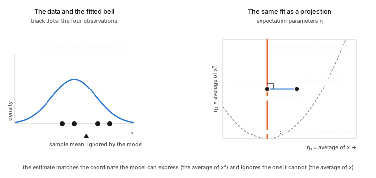
The observed point. Its \eta-coordinates are the averages of the two statistics: \bar\eta_1=\bar x=1 and \bar\eta_2=\overline{x^2}=(4+1+9+0)/4=3.5. This is a valid Gaussian point, because \bar\eta_2-\bar\eta_1^2>0 (the sample variance is positive).
The model. Zero-mean Gaussians have expectation parameters \eta=(0,\sigma^2): a vertical line in the \eta-plane.
The projection. The m-geodesic is a straight line in \eta and must meet the model at a right angle. The model only has freedom in the second coordinate, so the right angle forces the foot to match the second coordinate of the observed point: \hat\sigma^2=\overline{x^2}=3.5. The first coordinate of the data (the sample mean, 1) cannot be matched by the model and is ignored.
A check without geometry. The log-likelihood is -\frac N2\log\sigma^2-\frac{\sum x_i^2}{2\sigma^2}, and setting its derivative to zero gives \sigma^2=\frac1N\sum x_i^2=3.5: the same answer.

So the maximum likelihood estimate matches the dual coordinates that the model can express and ignores the rest: matching moments is the m-projection.

Why it is well behaved here. The zero-mean Gaussians form a straight line in \theta (\theta_1=\mu/\sigma^2=0), so the model is e-flat. By the projection theorem of Chapter 1, the m-projection onto an e-flat family is unique and gives the global minimum of the divergence. For a curved model the orthogonality condition only finds critical points, and local optima can appear.

Remarks in the book. Binomial and multinomial distributions are the exponential families that arise from the simplex by multiple observations. Many models of continuous data are only curved subfamilies of exponential families, where the same projection picture still applies, and a non-exponential model can be approximated locally by a larger exponential family.

The partition function

For an exponential family p(x;\theta)=\exp\{\theta\cdot x-\psi(\theta)\} with respect to a base measure \mu, the partition function is the normalising constant

Z(\theta)=\int e^{\theta\cdot x}\,d\mu(x)=e^{\psi(\theta)},

so the potential \psi of the earlier sections is its logarithm, \psi=\log Z.

Intuition. Start with the unnormalised score e^{\theta\cdot x} that the family gives to each outcome x. It says how favoured x is, but the scores do not add up to 1. To turn scores into probabilities, divide each by their total, and that total is Z(\theta): probability = score ÷ Z. The name comes from statistical physics, where the states of a system carry weights and Z sums the weights over all states.

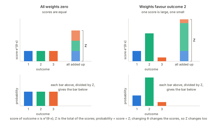
Two columns for two choices of weights on three outcomes. Top row: the unnormalised scores as coloured bars, with a stacked bar beside them whose total height is marked Z. Bottom row: each score divided by Z, giving the probabilities. With all weights zero the three scores are equal and so are the probabilities. When the weights favour outcome 2 its score is large, the total Z is larger, and the probabilities shift toward outcome 2. — Top: the scores e^{\theta\cdot x} and their total Z (the stacked bar). Bottom: each score divided by Z is a probability. Changing \theta changes the scores, and so changes Z as well.

Why it is more than a bookkeeping constant. Z depends on \theta, and that dependence holds everything about the family:

Slope gives the mean: \nabla\log Z=\mathbb E_\theta[x].
Curvature gives the covariance: \nabla^2\log Z=\operatorname{Cov}_\theta[x], which is the Fisher information, so \log Z is convex.
It is a Laplace transform of the base measure, which is why the inverse problem of recovering the measure from \psi (the book’s Theorem 2.2) is an inverse Laplace transform.
It must be finite. The family exists only for the \theta where the integral converges: for the Gaussian this is \theta_2<0.

Where it appeared above. For a coin or a softmax with one logit fixed at zero, Z=1+e^{\theta_1}+e^{\theta_2}, so \log Z is log-sum-exp and dividing by Z is the softmax. For the fixed-width Gaussian, completing the square gives Z=\sqrt{2\pi\sigma^2}\,e^{\sigma^2\theta^2/2}. And in the maximum entropy principle, Z is the normaliser that the Lagrange multipliers produce.

Names differ between texts. Amari’s \psi is the logarithm of the partition function. Machine-learning texts often say “partition function” for Z itself and “log-partition function” for \psi, and “free energy” for -\log Z in some conventions.

What an exponential family is: tilting a base distribution

An exponential family is a set of distributions that all share one form, in which the parameters meet the data only through a simple exponent:

p(x;\theta)=h(x)\,\exp\{\theta\cdot T(x)-\psi(\theta)\}.

\theta is the natural parameter (the knob, and the coordinates of the family).
T(x) is the sufficient statistic: the data affects the distribution only through T(x).
h(x) is a fixed base term that does not depend on \theta.
\psi(\theta) is the log-normaliser (\log Z of the previous section): whatever makes the total probability 1.

Intuition. Start from a base distribution h. Multiply each outcome by e^{\theta\cdot T(x)}, which favours outcomes with a large T(x) when \theta is positive and penalises them when it is negative, then divide by the total so it adds up to 1. Turning the knob \theta reshapes the distribution in this one structured way, and the family is the set of all such tilts.

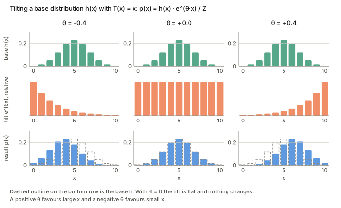
Three columns for theta equal to minus 0.4, 0 and plus 0.4. Top row: the same bump-shaped base distribution on the outcomes 0 to 10. Middle row: the tilt factor, which decays from left to right, is flat, or grows from left to right. Bottom row: the renormalised result, shifted toward small x, unchanged, or shifted toward large x, with a dashed outline of the base. — The same base h (top), the tilt e^{\theta x} (middle, drawn relative to its largest bar) and the result p (bottom, dashed outline is h). At \theta=0 nothing changes.

A measure on the sample space absorbs h

The book removes h from the formula by moving it into the measure that the density is taken against. Define a measure on the sample space X by

d\mu(x)=e^{k(x)}\,dx,\qquad\text{so that } e^{k}=h .

This is the idea from the measure page that a function builds a measure: \mu(A)=\int_A e^{k(x)}dx gives each region the weight e^{k} instead of the same weight everywhere, and e^{k} is the density of \mu with respect to the ordinary dx. Probabilities are then P(A)=\int_A\exp\{\theta\cdot x-\psi(\theta)\}\,d\mu(x), which is the same as before, but the density against \mu has the bare form \exp\{\theta\cdot x-\psi\}. The normaliser is e^{\psi(\theta)}=\int e^{\theta\cdot x}d\mu(x).

Two remarks. For a discrete family \mu is a sum instead of an integral; for the Poisson family h(x)=1/x! is just a weight of 1/x! on each integer x. And writing the statistic as x itself loses nothing: rename y=T(x) and work with y.

The usual families in exponential-family form

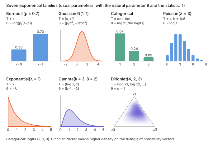
Each line takes the usual formula, takes its log, and sorts the terms into the part that depends on x only (h), the part where \theta meets x (\theta\cdot T) and the part that depends on the parameters only (-\psi).

Family	Usual form	T(x)	Natural parameter \theta	h(x)	\psi(\theta)
Bernoulli	p^x(1-p)^{1-x}	x	\log\frac{p}{1-p}	1	\log(1+e^{\theta})
Gaussian	\frac{1}{\sqrt{2\pi\sigma^2}}e^{-(x-\mu)^2/2\sigma^2}	(x,x^2)	\big(\frac{\mu}{\sigma^2},-\frac{1}{2\sigma^2}\big)	1	-\frac{\theta_1^2}{4\theta_2}+\frac12\log\frac{\pi}{-\theta_2}
Categorical	P(x=k)=\pi_k	one-hot	\theta_k=\log\pi_k (logits)	1	\log\sum_j e^{\theta_j}
Poisson	\frac{\lambda^x e^{-\lambda}}{x!}	x	\log\lambda	\frac1{x!}	e^{\theta}
Exponential	\lambda e^{-\lambda x}	x	-\lambda	1	-\log(-\theta)
Gamma	\frac{\beta^k}{\Gamma(k)}x^{k-1}e^{-\beta x}	(\log x,x)	(k-1,-\beta)	1	\log\Gamma(\theta_1{+}1)-(\theta_1{+}1)\log(-\theta_2)
Dirichlet	\frac{\Gamma(\sum\alpha_i)}{\prod\Gamma(\alpha_i)}\prod x_i^{\alpha_i-1}	(\log x_i)	\alpha_i-1	1	\sum\log\Gamma(\alpha_i)-\log\Gamma(\sum\alpha_i)

For example, the Bernoulli: p^x(1-p)^{1-x}=\exp\{x\log\frac{p}{1-p}+\log(1-p)\}, so \theta=\log\frac{p}{1-p} (the log-odds), \psi=-\log(1-p), and the sigmoid is the map from \theta back to p. For the Gaussian, expand the square: the exponent is \frac{\mu}{\sigma^2}x-\frac{1}{2\sigma^2}x^2-\frac{\mu^2}{2\sigma^2}-\frac12\log(2\pi\sigma^2). The categorical’s logits are defined only up to adding one constant to all of them, so the “minimal” version fixes one class to zero.

Seven small plots: Bernoulli as two bars, a Gaussian bell, categorical as three bars, Poisson as bars from 0 to 9, a decaying exponential curve, a gamma hump, and a Dirichlet density shaded on a triangle. Each has its sufficient statistic and natural parameter written above. — One member of each family from the table, with its sufficient statistic T and natural parameter \theta.

Theorem 2.1: the Fisher metric is the curvature of \psi

The theorem says that the Riemannian metric of an exponential family is the Fisher information matrix,

g_{ij}(\theta)=E\big[\partial_i\log p(x;\theta)\,\partial_j\log p(x;\theta)\big],\qquad\partial_i=\frac{\partial}{\partial\theta^i}.

A Riemannian metric is a rule for the length of a small step: ds^2=\sum g_{ij}\,d\theta^i d\theta^j, with g allowed to change from point to point. Here the rule measures how distinguishable p(x;\theta) is from p(x;\theta+d\theta). For an exponential family it also has an explicit form, obtained in five short steps:

Take the log: \log p=\theta\cdot x-\psi(\theta)+k(x).
Differentiate in \theta (the score): the k(x) term drops out and \partial_i\log p=x_i-\partial_i\psi.
Use E[x_i]=\partial_i\psi=:\eta_i, so the score is the data minus its mean, x_i-\eta_i.
Put it in the definition: g_{ij}=E[(x_i-\eta_i)(x_j-\eta_j)]=\operatorname{Cov}(x_i,x_j).
Differentiating E[x]=\nabla\psi once more gives \operatorname{Cov}(x)=\nabla^2\psi.

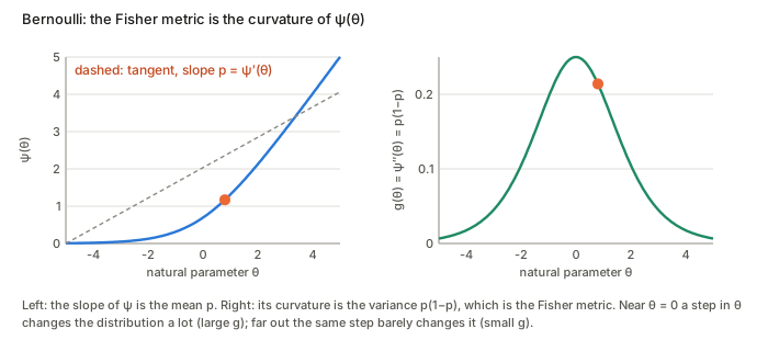
So the Fisher metric is the covariance matrix of the statistic, and equally the Hessian of \psi; since a covariance matrix is positive semi-definite, \psi is convex and g is a genuine metric. For the Bernoulli, \psi'=p and \psi''=p(1-p), the variance of a coin.

Left: the curve psi of theta for the Bernoulli family, rising from near zero on the left to a straight rise on the right, with a dashed tangent line at a marked point. Right: the second derivative p times one minus p, a bell-shaped curve peaking at theta equal to zero, with the same point marked. — Left: \psi(\theta)=\log(1+e^{\theta}), whose slope at a point is the mean p. Right: its curvature g(\theta)=p(1-p), the Fisher metric, which is largest at \theta=0. A step of fixed size in \theta is a long statistical distance near 0 and a short one far out.

Mixture families

A mixture family is a set of distributions built by blending a few fixed ingredients with adjustable weights. Take fixed distributions p_0(x),p_1(x),\dots,p_n(x) on the same space and let

p(x;\eta)=\sum_{i=0}^{n}\eta_i\,p_i(x),\qquad\eta_i\ge0,\ \ \sum_i\eta_i=1 .

There are n free weights (the last is fixed by \eta_0=1-\sum_{i\ge1}\eta_i), so the family is an n-dimensional manifold with the weights \eta as coordinates.

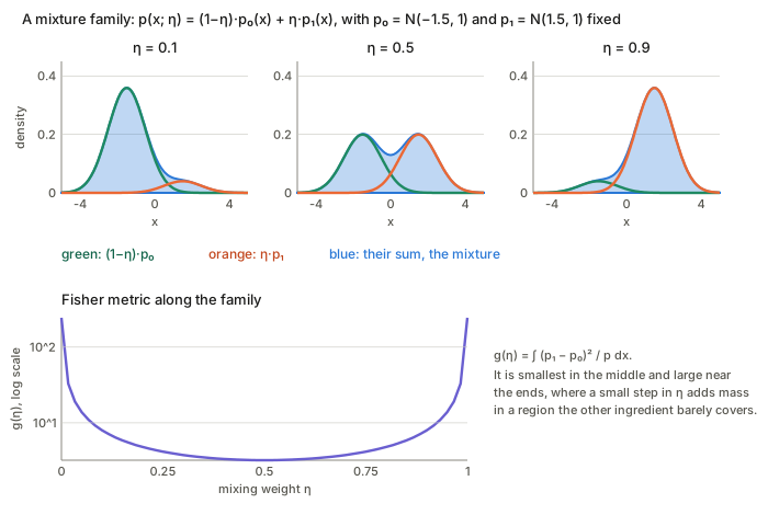
Top: three plots for mixing weights 0.1, 0.5 and 0.9, each showing the weighted left Gaussian in green, the weighted right Gaussian in orange and their sum in blue, which is one hump on the left, two humps, then one hump on the right. Bottom: the Fisher metric along the mixing weight on a log scale, a U-shaped curve that is smallest at 0.5 and large at both ends. — Two fixed Gaussians p_0=N(-1.5,1) and p_1=N(1.5,1) blended with weights 1-\eta and \eta. The ingredients never change; only their weights do. Below, the Fisher metric g(\eta)=\int(p_1-p_0)^2/p\,dx along the family: small in the middle, large near the ends, where a small step in \eta adds mass in a region the other ingredient barely covers.

Why it is a clean geometric object. The family is linear in the probabilities: averaging two members’ densities gives the member whose weights are the average of theirs. So “straight lines” here are straight when you average probabilities. This is the m-flat (mixture-flat) structure, the counterpart of the e-flat structure of exponential families, which is straight in \log p.

	Exponential family	Mixture family
Form	p=h\,e^{\theta\cdot T-\psi}	p=\sum_i\eta_i\,p_i
Linear in	\log p	p
Coordinates	natural \theta	mixture weights \eta
Flat structure	e-flat	m-flat

The set of all categorical distributions on n+1 outcomes is both: a mixture of the point masses \delta_i, with the weights as coordinates, and an exponential family in the softmax form. It is the one family where both flat structures coexist.

A common confusion. A “Gaussian mixture model” whose means and variances are also learned is not a mixture family in this sense. Here the ingredients p_i are fixed and only the weights vary. Learning the Gaussian centres too gives a larger, curved model, flat in neither direction.