Kernel functions: similarity that behaves like a dot product

kernelpositive-definite-kernelgram-matrixkernel-trickfeature-spacerkhskernel-exponential-family

In one paragraph

A kernel function k(x,y) takes two points and returns a number saying how similar they are: large when x and y are close or alike, small when they are far apart. A positive definite kernel is one that is guaranteed to behave like a dot product, k(x,y)=\langle\varphi(x),\varphi(y)\rangle, of some feature vectors \varphi(x) that live in a (possibly infinite-dimensional) space. The kernel trick is that you can take that dot product with a formula in the original space, without ever building the feature vectors. The kernel exponential family uses a kernel to turn a weight function \theta(y) into a smooth log-density.

What a kernel looks like

For a fixed y, the function x\mapsto k(x,y) is a bump placed at y. The standard example is the Gaussian kernel

k_\sigma(x,y)=\exp\Big\{-\frac{(x-y)^2}{2\sigma^2}\Big\},

a bump of width \sigma around y: a small \sigma gives a narrow bump (only nearby points count as similar), a large \sigma a wide one. Other kernels are the linear kernel x\cdot y, the polynomial kernel (x\cdot y+1)^d, and, as the extreme case, the delta function \delta(x-y), which is 1 at x=y and 0 elsewhere.

Positive definite: the Gram-matrix test

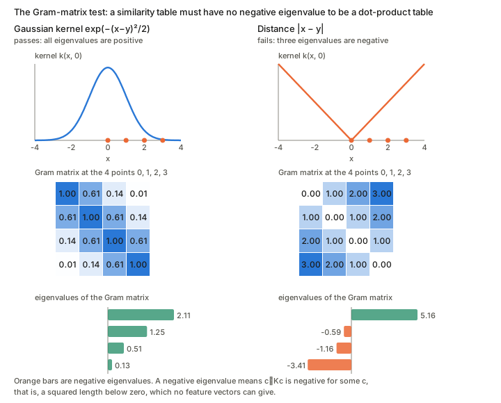
Pick any finite list of points x_1,\dots,x_n and write the table of all their similarities, the Gram matrix K_{ij}=k(x_i,x_j). The kernel is positive (semi-)definite if K is a positive (semi-)definite matrix for every choice of points, that is, if

\sum_{i,j}c_ic_j\,k(x_i,x_j)\ \ge 0\quad\text{for all numbers }c_1,\dots,c_n .

Letting the points fill the line, the sum becomes the integral \iint k(x,y)f(x)f(y)\,dx\,dy>0 for every function f\neq0, which is the condition the book states for the kernel exponential family. This is the matrix condition of the positive definite matrices page applied to similarity tables.

Two columns. Left: the Gaussian kernel as a bell curve, its four by four Gram matrix shaded dark on the diagonal and fading away from it, and four green eigenvalue bars that are all positive. Right: the distance kernel as a V shape, its Gram matrix shaded darker away from the diagonal, and eigenvalue bars with one large green bar and three orange negative bars. — The same test on two kernels at the points 0,1,2,3. The Gaussian kernel gives a table whose eigenvalues are all positive. The distance |x-y| gives a table with negative eigenvalues (orange), so it is not a valid kernel, even though it measures how far apart two points are.

Why a negative eigenvalue rules out a dot product

Suppose k(x,y)=\langle\varphi(x),\varphi(y)\rangle. For any numbers c_i, collect the vectors into one vector v=\sum_i c_i\varphi(x_i). Then

c^\top Kc=\sum_{i,j}c_ic_j\langle\varphi(x_i),\varphi(x_j)\rangle=\Big\langle\sum_ic_i\varphi(x_i),\sum_jc_j\varphi(x_j)\Big\rangle=\|v\|^2\ \ge 0 .

So a table of dot products can never give a negative c^\top Kc, which is the squared length of a vector. If u is an eigenvector of K with eigenvalue \lambda, then u^\top Ku=\lambda\|u\|^2, so a negative eigenvalue would give a negative squared length. That is impossible, so no feature vectors exist. The converse holds as well (Mercer, Moore–Aronszajn): if no eigenvalue is ever negative, write K=Q\Lambda Q^\top and take the rows of Q\Lambda^{1/2} as the feature vectors.

A passing result on one set of points proves nothing about the kernel in general, since it has to pass for every set of points; a single negative eigenvalue on any set is enough to rule a kernel out.

Why not just use “1 minus the distance”?

A distance measures dissimilarity, so 1-|x-y| looks like a natural similarity, but it fails as soon as two points are more than 2 apart (the similarity becomes negative so badly that the two-point table has a negative eigenvalue). The reason is that subtracting a distance does not respect the dot-product structure. If k is a dot product with k(x,x)=1, then the squared distance between the feature vectors is

\|\varphi(x)-\varphi(y)\|^2=k(x,x)+k(y,y)-2k(x,y),\qquad\text{so}\qquad k(x,y)=1-\tfrac12\|\varphi(x)-\varphi(y)\|^2 .

The correct “one minus distance” subtracts half the squared distance between feature vectors, not a distance measured in the input space. The usual way to turn a distance into a valid similarity is to exponentiate the squared distance, as in the Gaussian kernel (Schoenberg’s theorem says exactly when this works).

The kernel trick: never build the feature space

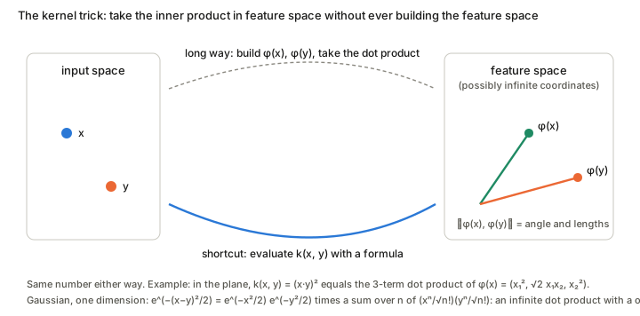
On the left a box for the input space with two points x and y. On the right a box for the feature space with two arrows from a common origin for phi of x and phi of y. A dashed arc above is labelled long way: build the feature vectors and take their dot product. A solid arc below is labelled shortcut: evaluate the kernel k of x and y with a formula. — Two routes to the same number. The long route maps x and y into the feature space and takes the dot product there. The shortcut evaluates a closed-form kernel in the input space.

The infinite dimension does not go away: it is where the dot product lives. The trick is that the dot product has a closed form, so you never write the coordinates.

A finite example. In the plane, k(x,y)=(x\cdot y)^2=x_1^2y_1^2+2x_1x_2y_1y_2+x_2^2y_2^2 is the dot product of \varphi(x)=(x_1^2,\sqrt2\,x_1x_2,x_2^2). Computing the kernel needs one dot product and a square, whichever the size of the feature space.
The infinite case is the same. In one dimension, e^{-(x-y)^2/2}=e^{-x^2/2}e^{-y^2/2}e^{xy} and e^{xy}=\sum_n\frac{x^n}{\sqrt{n!}}\frac{y^n}{\sqrt{n!}}, a dot product of two infinite vectors. The infinite sum collapses into one exponential.
Algorithms only need the table. Kernel regression, SVMs and the like use only inner products between the feature vectors of the data points, that is, the n\times n Gram matrix. The representer theorem says the best solution lies in the span of \varphi(x_1),\dots,\varphi(x_n), so everything is a finite computation with n numbers. The price is that the cost grows with the number of data points rather than with the feature dimension.

Positive definiteness is what guarantees that the hidden feature space exists. A kernel that fails the Gram test has no feature space, and the trick would give meaningless answers.

The reproducing kernel Hilbert space

A reproducing kernel Hilbert space (RKHS) is the space of functions you can build by adding up bumps of a positive definite kernel, with a dot product chosen so that evaluating a function at a point is itself a dot product. It is the feature space of the kernel trick, made concrete as a space of functions.

Functions made of bumps. For each point y, k(\cdot,y) is a bump centred at y. The RKHS H_k is the set of weighted sums of bumps (and their limits),

f(x)=\sum_ic_i\,k(x,x_i).

This is the same “smear weights through the kernel” construction as f(x)=\int\theta(y)k(x,y)\,dy in the kernel exponential family: those f are elements of this space.

A dot product on functions. Require the bumps to act like the feature vectors, \langle k(\cdot,x),k(\cdot,y)\rangle=k(x,y), and extend linearly. For f=\sum_ic_ik(\cdot,x_i) this gives

\|f\|^2=\sum_{i,j}c_ic_j\,k(x_i,x_j)=c^\top Kc,

the quantity of the Gram-matrix test. Positive definiteness of k is what makes this a genuine squared length. (“Hilbert” means a space with such an inner product that has no gaps: every sequence that settles down has a limit in the space.)

The reproducing property. Take the inner product of f with a single bump:

\langle f,k(\cdot,x)\rangle=\sum_ic_ik(x_i,x)=f(x).

Evaluating f at x is the same as taking a dot product with the bump at x. That is the “reproducing” in the name, and it is the kernel trick in function form: the feature vector of the point x is the bump \varphi(x)=k(\cdot,x), and \langle\varphi(x),\varphi(y)\rangle=k(x,y).

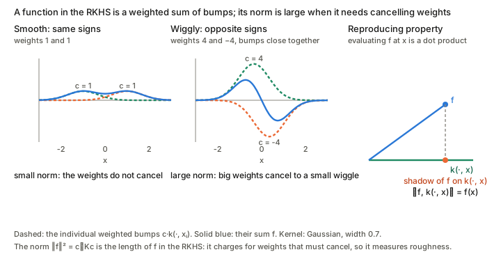
Left and middle: a function in the RKHS is a weighted sum of bumps (dashed), and its norm c^\top Kc is small when the weights do not cancel and large when large weights have to cancel to make a small wiggle. Right: the reproducing property, drawn as a projection: the shadow of f on the bump at x has the value f(x).

Why this is more than a convenience. In an ordinary function space, two functions can be close in length but differ wildly at one point, so evaluating at a point is not a well-behaved operation. In an RKHS, evaluation is continuous: |f(x)|\le\|f\|\sqrt{k(x,x)}, so a small norm means small values everywhere. This property characterises these spaces: every positive definite kernel has such a space, and every Hilbert space of functions with continuous evaluation has such a kernel (the Moore–Aronszajn theorem).

The norm measures roughness. With a Gaussian kernel, a function that wiggles quickly can only be made from large cancelling weights, so it has a big norm, while a smooth function has a small one. Kernel methods exploit this by minimising a fit error plus \lambda\|f\|^2, which prefers smooth fits. It is also why a wide kernel allows only smooth functions, as in the kernel-smoothing figure of the kernel exponential family section.

Where it appears

In the kernel exponential family, \int\theta(y)k(x,y)\,dy is an element of the RKHS and an inner product in the feature space, with \theta the weights, so the family is an ordinary exponential family with a function-valued parameter. The positivity of the kernel is what makes \psi[\theta] convex.