Bayesian Evidence and Model Selection
Links
- arXiv:1411.3013 — preprint (v2, November 2015, the version these notes follow). Published in Digital Signal Processing 47, a special issue for W. J. Fitzgerald.
- Interactive companion — three widgets: the Occam factor with sliders, a nested-sampling run you can step through, and the importance-sampling ratio estimator next to the version printed as eq. (38).
- The ELBO — the background page for section 4.6 (variational Bayes): the same identity \log Z = \text{bound} + \mathrm{KL}, there called the ELBO.
- Expectation–Maximization — the same “lower bound plus a KL gap” idea, for point estimates.
- Langevin dynamics — the Gibbs law e^{-U/D} behind the statistical-physics analogy of section 4.3.
- Code — only the script that draws the figures. The code blocks below are for reading; the notes quote no output from running them.
In one paragraph
To compare two theories (families of models) M_1 and M_2 against data d, Bayes’ theorem says the posterior odds equal the prior odds times a ratio of evidences Z_k = P(d\mid M_k), the probability each theory assigned to the data averaged over its own prior. That average is the whole story: a theory is rewarded for fitting, and punished for having spread its prior over many parameter values that fit badly. The punishment is the Occam factor, and it is automatic. The catch is that Z is an integral over the whole parameter space, almost never solvable. The paper is a tour of ways to estimate it: replace the integrand by a Gaussian (Laplace), sample from a stand-in (importance sampling), slowly turn the likelihood on (thermodynamic integration, annealed importance sampling), lower-bound it with a simpler distribution (variational Bayes), or sweep the likelihood from the top down (nested sampling). Four applications close it: signal detection, a light sensor, exoplanet light curves, and force fields for proteins.
It is a review, so there is little to “prove” in the sense of a new theorem. What is worth doing, and what these notes do, is work each derivation line by line, say what each step buys, and check the equations as printed. Several have small slips (collected in Questions and doubts), and one application claim looks hard to square with the paper’s own formulas.
The spine of the argument
- Posterior odds of two theories = prior odds × Bayes factor, and the Bayes factor is a ratio of evidences (section 2).
- An evidence is a likelihood averaged over the prior, so it equals best fit × Occam factor, where the Occam factor is the fraction of the prior that fits the data (section 3).
- Computing the evidence integral is the hard part, and each method
trades one difficulty for another (section 4):
- Laplace: assume the integrand is a Gaussian bump. Cheap and exact for Gaussians; wrong for skewed or multi-peaked integrands.
- Importance sampling: reweigh samples from an easy distribution. Fine only if the weights stay tame.
- Thermodynamic integration / AIS: connect an easy distribution (the prior) to the hard one (the posterior) through a path, and accumulate the change in normaliser along the path.
- Variational Bayes: the evidence is bounded below by a computable quantity, and the slack is a KL.
- Nested sampling: turn the many-dimensional integral into a one-dimensional integral over prior mass, and estimate the mass by counting how fast a cloud of points shrinks.
- Examples show each use: the evidence picking between “signal” and “no signal”, between numbers of Gaussians, between physical effects, between force fields (section 5).
Setup and notation
| Symbol | Meaning |
|---|---|
| d | the data |
| m | one particular model (a parameter value) inside a theory |
| M (or M_1, M_2) | a theory: a family of models, e.g. “a line” or “a quadratic” |
| I | all background information, written to the right of the bar |
| P(m\mid M,I) | prior over parameters inside the theory |
| P(d\mid m,M,I) | likelihood, written L(m) |
| Z = P(d\mid M,I) | the evidence (also the marginal likelihood) |
| \mathrm{OR} | the odds ratio or Bayes factor Z_1/Z_2 |
Two warnings about words. First, “model selection” here means choosing a theory (a whole family), not a parameter value. Choosing a parameter value is parameter estimation, where the evidence is only the normalising constant and can be ignored. Second, the abstract calls Bayes factors “also known as log odds ratios”: the Bayes factor is the ratio, its logarithm is the log odds ratio, and neither is the posterior odds unless the prior odds are one.
From Bayes’ theorem to the odds ratio (section 2)
Start with the product rule written two ways, P(m,d\mid M)=P(m\mid M)P(d\mid m,M)=P(d\mid M)P(m\mid d,M) (eqs. 1–3). Equate and divide:
P(m\mid d,M)=P(m\mid M)\,\frac{P(d\mid m,M)}{P(d\mid M)}.
The denominator is whatever makes the left side add up to one, so
Z=P(d\mid M)=\int dm\,P(m\mid M)\,P(d\mid m,M)\qquad\text{(eqs. 5–6)}.
That is where the name marginal likelihood comes from: the parameter has been integrated out.
For two theories, apply the product rule to the joint P(M_k,d\mid I) both ways and divide the two cases (eqs. 7–9):
\frac{P(M_1\mid d,I)}{P(M_2\mid d,I)}=\frac{P(M_1\mid I)}{P(M_2\mid I)}\times\underbrace{\frac{Z_1}{Z_2}}_{\mathrm{OR}}.
The factor P(d\mid I) appears in both joints and cancels, which is why it never matters. (Eq. 7 as printed has the same expression on both sides of the equals sign, a typo: the left side should be P(M_1,d\mid I)/P(M_2,d\mid I), the right side the first line of eq. 8.)
Intuition. Each theory makes a bet: “if I am right, the data will look like this”. The evidence is how much probability each theory put on what was actually seen. The odds ratio compares the two bets.
Occam’s razor falls out (section 3)
Take one parameter x with a flat prior over a width \Delta x. Let L_{\max} be the best likelihood value, and define the effective width of the likelihood as the width of a rectangle of height L_{\max} that has the same area (eq. 13):
\delta x=\frac{1}{L_{\max}}\int L(x)\,dx .
Then, because the prior density is the constant 1/\Delta x,
Z=\frac{1}{\Delta x}\int L(x)\,dx=L_{\max}\,\frac{\delta x}{\Delta x}=L_{\max}\,W,\qquad 0\le W\le1\qquad\text{(eqs. 14–17)}.
So evidence = best fit × Occam factor, and the Occam factor W is the fraction of the prior that is compatible with the data.
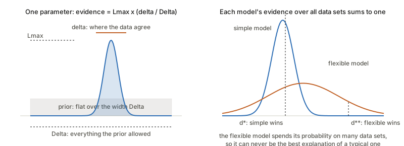
Read the left panel as a competition for a fixed budget. The prior has one unit of probability to hand out, and spreads it evenly. A bigger \Delta x means each parameter value gets less, so the same likelihood bump earns less evidence. “By making the prior broader we pay in evidence.”
The right panel is the more useful picture (it is the standard one from MacKay’s textbook, not drawn in this paper). Fix a theory. Its evidence is a probability distribution over data sets: it must integrate to one over everything the theory could have predicted. A flexible theory can fit many data sets, so it spreads its one unit thinly. A rigid theory fits few data sets, but puts a lot of weight on those. If the data land where the rigid theory said they would, it wins by a lot; if the data land where only the flexible theory could have gone, the flexible one wins. Nothing penalises complexity by decree. It is a consequence of normalisation.
More parameters mean more factors: if each of K extra parameters has the same ratio \delta x/\Delta x, the Occam factor behaves like (\delta x/\Delta x)^K. Once the fit cannot improve any further, adding parameters only costs.
A Gaussian worked in full (eqs. 18–19)
With n independent observations of a quantity with known noise level \sigma, the likelihood depends on the data only through the sample mean \bar d and sample variance v:
L(x)=(2\pi\sigma^2)^{-n/2}\exp\!\Big\{-\tfrac{n}{2\sigma^2}\big[(x-\bar d)^2+v\big]\Big\}.
(Expand \sum_i(x-d_i)^2=n(x-\bar d)^2+nv to see it.) As a function of x this is a Gaussian centred at \bar d with standard deviation \sigma/\sqrt n, and L_{\max} is its peak value. Its area is the peak times \sqrt{2\pi}\,\sigma/\sqrt n, so if the prior range comfortably contains the bump,
W=\frac{\sqrt{2\pi}\,\sigma}{\Delta x\,\sqrt n}.
This reads well. The bump gets narrower as the data increase (\sqrt n), so the Occam factor shrinks with more data. That is not a bug: with more data you have learnt the parameter more precisely, and you are paying for having specified it so tightly out of the prior range. A theory with a free parameter has to be worth that cost.
The odds ratio between a theory with no free parameter (M_0) and one with x free (M_1) is then \mathrm{OR}\approx\frac{L(M_0)}{L_{\max}}\cdot\frac{\Delta x}{\delta x} (eq. 20): a likelihood ratio, the only thing a frequentist likelihood-ratio test uses, times an Occam factor the test leaves out.
Why computing Z is hard
Z is an integral of prior × likelihood over all parameters. Nothing is wrong with the integral; the trouble is that nearly all of the integrand’s mass sits in a tiny region that you do not know the location or shape of, in a space with many dimensions. Averaging the likelihood over prior samples nearly never lands in that region. Posterior samples (from MCMC) land there, but they say nothing about the normalising constant, because MCMC never needs it. Every method below is a way around this.
Laplace approximation (section 4.1)
Idea. Near its peak, any smooth log-density looks like a downward parabola, and a parabola in the log is a Gaussian. A Gaussian’s integral is known.
Expand \ln p around the peak x_0, where the slope is zero (eq. 22):
\ln p(x)\simeq\ln p(x_0)+\tfrac12(\ln p)''(x_0)\,(x-x_0)^2 .
The curvature is negative at a maximum, so define the width through \sigma^2=-1/(\ln p)''(x_0). Then p(x)\simeq p(x_0)\exp\{-(x-x_0)^2/2\sigma^2\} and
Z=\int p\simeq p(x_0)\sqrt{2\pi\sigma^2}.
In N dimensions the curvature becomes the Hessian A_{ij}=-\partial_i\partial_j\ln p(x_0) and (eq. 30)
Z\simeq p(x_0)\sqrt{\frac{(2\pi)^N}{\det A}} .
With p = prior × likelihood, this is the evidence. Look at the shape: \sqrt{(2\pi)^N/\det A} is the volume of the Gaussian bump, so Laplace is “peak height × peak volume”, the same L_{\max}\cdot W decomposition as before, now with the bump volume measured by the curvature at the top. Sharper curvature means a bigger \det A and a smaller bump.
Where it fails. Skewed peaks, several peaks, a ridge that is not Gaussian-shaped. It is also exact when the integrand is Gaussian (then there is no approximation at all), which is why it is the base of richer schemes such as the evidence framework and INLA.
(Eq. 23 as printed has an extra \tfrac12 inside \sigma^2=-\big(\tfrac12(\ln p)''\big)^{-1}, which would make \sigma^2 twice too large. See the doubts.)
import numpy as np

def laplace_log_evidence(log_p, x0, hessian):
    """log Z for p(x) = prior * likelihood, given the mode x0 and the Hessian of -log p there."""
    N = len(x0)
    sign, logdet = np.linalg.slogdet(hessian)
    return log_p(x0) + 0.5 * N * np.log(2 * np.pi) - 0.5 * logdet
Importance sampling (section 4.2)
Idea. To average f under a hard distribution p, sample from an easy distribution q and correct each sample by the weight p/q. Rewrite p=\frac pq\,q (the only requirement is that q>0 wherever p>0):
\langle f\rangle_p=\frac{\int f\,\frac pq\,q}{\int\frac pq\,q}\;\approx\;\frac{\sum_i f(x_i)\,p(x_i)/q(x_i)}{\sum_i p(x_i)/q(x_i)},\qquad x_i\sim q\qquad\text{(eqs. 32–34)}.
The denominator is what lets p be unnormalised.
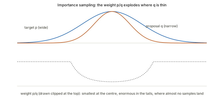
Why the weights must stay tame: the tails of p are exactly where q is rare, so the few samples that land there carry enormous weights, and a handful of those dominate the sum. The estimate then depends on whether one lucky sample showed up. A proposal narrower than the target is dangerous for just that reason.
The estimator for a ratio of evidences (eqs. 35–38). Writing Z_p=\int p, Z_q=\int q and sampling x_i from the normalised q/Z_q, the right estimator is the plain average of the weights:
\frac{Z_p}{Z_q}=\int\frac pq\cdot\frac q{Z_q}\;\approx\;\frac1N\sum_i\frac{p(x_i)}{q(x_i)} .
The paper’s eq. (38) instead prints \sum_i p^2(x_i)/q^2(x_i)\big/\sum_i p(x_i)/q(x_i). That looks like eq. (34) applied with f=p/q, and eq. (34) averages under p, not under q, so it estimates a different quantity. A two-point example shows it is not the same: if the weight p/q takes the value 1 or 3 with equal chance under q, the correct estimate tends to 2, while (38) tends to 10/4. See the interactive page, which runs both. (A natural reading is a typo; the thing written in eq. 37, \langle p/q\rangle_q, is right.)
The statistical-physics dictionary (section 4.3)
Physics integrates a Boltzmann weight e^{-\beta E(x)} over all configurations x to get the partition function Z(\beta)=\int dx\,e^{-\beta E(x)}. Evidence is the same integral:
| Physics | Bayes |
|---|---|
| configuration x | parameter m |
| energy E(x) | -\log L(m) |
| inverse temperature \beta | exponent on the likelihood |
| partition function Z(\beta{=}1) | the evidence |
| density of states g(E) | prior mass at each energy level |
The density of states g(E)=\int dm\,P(m)\,\delta[E-E(m)] says how much prior mass sits at energy E (eq. 42). Group the integral by energy level and the evidence collapses to one dimension (eq. 43):
Z=\int dE\,g(E)\,e^{-E}.
Why this is a big deal. A 10^3-dimensional integral has become a one-dimensional one, provided you can find g(E). Everything else in the paper is two families of ways to do that. Thermal methods (sections 4.4, 4.5) raise the likelihood to a power \beta and slide it from 0 to 1, P(m)\,L(m)^\beta (eq. 44), bridging the prior (\beta=0) and the posterior (\beta=1). Nested sampling (4.7) estimates g directly.
Thermodynamic integration (section 4.4)
Idea. Instead of Z(1) itself, estimate the change in \log Z as \beta moves from 0 to 1, by integrating a slope that samples can measure.
Take the path p(x\mid\beta)\propto p_0^{1-\beta}p_1^\beta with normaliser Z(\beta)=\int p_0^{1-\beta}p_1^\beta. Differentiate \log Z:
\partial_\beta\log Z=\frac1{Z(\beta)}\int p_0^{1-\beta}p_1^\beta\,\log\frac{p_1}{p_0}\,dx=\Big\langle\log\frac{p_1}{p_0}\Big\rangle_\beta\qquad\text{(eq. 47)}.
The derivative of a log-normaliser is an average of what the parameter multiplies in the exponent: the standard trick. Integrate from 0 to 1 and split into slices (eqs. 48–49):
\log\frac{Z(1)}{Z(0)}=\int_0^1\Big\langle\log\frac{p_1}{p_0}\Big\rangle_\beta\,d\beta\;\approx\;\sum_i\Big\langle\log\frac{p_1}{p_0}\Big\rangle_{\beta_i}(\beta_{i+1}-\beta_i).
For evidence take p_0= prior (so Z(0)=1) and p_1= prior × likelihood (so Z(1)= evidence), and the integrand is the average log-likelihood under the tempered posterior.
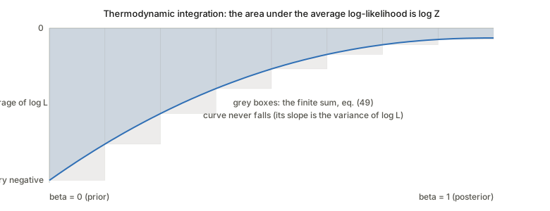
Three things to notice. The curve never falls: its slope is the variance of the log-likelihood under p(\cdot\mid\beta), which cannot be negative (differentiate \langle\log L\rangle_\beta once more). The curve starts at the average log-likelihood under the prior, which is typically very negative, so the area is a large negative number: \log Z is mostly a cost, the Occam penalty, paid when you compress from the prior to the posterior. And the rectangles only follow the curve well if the steps are placed where it moves. The paper flags this as an open difficulty for systems with phase transitions, and mentions ensemble annealing (choose each next \beta so that the KL divergence between consecutive distributions is constant) as a response.
If the two theories share parameters, the same machinery run between the two posteriors (eqs. 50–51) estimates the log odds ratio directly, with no need for either evidence alone.
Annealed importance sampling (section 4.5)
Thermodynamic integration estimates \log(Z_1/Z_0) and then exponentiates; the result is generally biased. AIS estimates the ratio itself without bias.
Run a chain of intermediate distributions p_0,p_1,\dots,p_n (for example along the geometric path). Each run j generates states x_1^{(j)},\dots, where x_i comes from a Markov step that leaves p_i invariant, started from x_{i-1}. Give the run the weight (eq. 53)
w^{(j)}=\prod_i\frac{p_{i+1}(x_i^{(j)})}{p_i(x_i^{(j)})} .
Neal’s result: \mathbb E[w]=Z_1/Z_0 exactly, whether or not the chain has equilibrated. A sketch of why: the whole run is one big sample from a joint distribution over the path (x_0,x_1,\dots). Pair it with a “reverse” joint in which the same states are generated backwards, started from p_1. Each forward transition is invariant for p_i, so each factor turns into a term of a plain importance weight between the reversed and forward joints, and the telescoping product of ratios is w. The reverse joint has total mass Z_1 and the forward one Z_0, so \mathbb E[w]=Z_1/Z_0.
Arithmetic against geometric mean (eqs. 55–58). The AIS estimate is the arithmetic mean \frac1M\sum_j w^{(j)}. Doing thermodynamic integration on the same runs and exponentiating gives \exp\big(\frac1M\sum_j\log w^{(j)}\big), the geometric mean of the same weights. By the arithmetic–geometric inequality the geometric mean is never larger, so the exponentiated thermodynamic-integration estimate sits at or below AIS, and the gap grows with the spread of \log w. The paper does not say which side the bias is on; it is on the low side (Jensen).
Variational Bayes (section 4.6)
Idea. Do not try to compute \log Z; build a number that is below it and that you can compute, and push it up.
Take any density Q(m). Because Q integrates to one, \log Z=\int Q(m)\log Z\,dm (eq. 60). Use Z=P(d,m)/P(m\mid d) (the product rule again), multiply and divide by Q, and split the log (eqs. 61–65):
\log Z=\underbrace{\int Q\log\frac{P(d,m)}{Q}}_{F(Q)\ \text{(negative free energy)}}+\underbrace{\int Q\log\frac{Q}{P(m\mid d)}}_{\mathrm{KL}[Q\,\|\,P(m|d)]}.
The first term needs only the joint, never the evidence. The second is a KL divergence, always \ge0, and zero only when Q is the posterior. So F(Q)\le\log Z for every Q, with equality at the posterior (eq. 66). This is the same identity as the ELBO; the paper’s “negative free energy” is the ELBO, and “ensemble learning” is an old name for the same method.
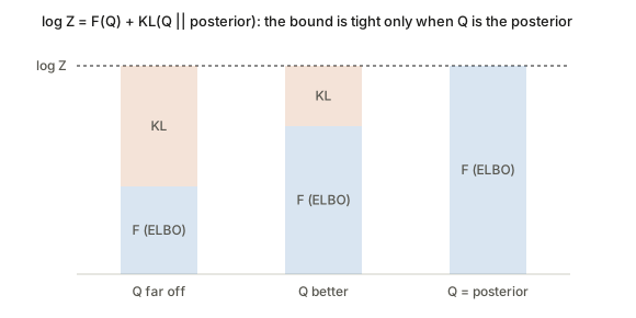
The total never changes; maximising F and minimising the KL are the same act. You cannot minimise the KL directly because it contains the unknown P(m\mid d). You can raise F.
The mean-field step (eqs. 67–70). To make F tractable, restrict Q to a product Q(m_0)Q(m_1). Holding Q(m_1) fixed and collecting the terms involving m_0,
F=\int Q(m_0)\,\mathcal I(m_0)\,dm_0-\int Q(m_0)\log Q(m_0)\,dm_0+C,\qquad\mathcal I(m_0)=\int Q(m_1)\log P(d,m_0,m_1)\,dm_1 .
Writing \mathcal I=\log e^{\mathcal I} puts this in KL form, and the best Q(m_0) is proportional to e^{\mathcal I(m_0)} (eq. 70): the optimal factor is the average of the log-joint over the other factors, exponentiated. Alternate, one factor at a time. This is “coordinate ascent”, and each pass raises F.
Two cautions, both visible in the paper’s text. Eq. (69) as printed reads F=\mathrm{KL}[\cdot]+C and then says F is “minimised” at the optimum. With the signs as derived it should be F=-\mathrm{KL}+C, so F is maximised when the KL vanishes. The closing sentence of the section (“estimated by minimizing the negative free energy”) has the same slip. And a product-form Q cannot equal a posterior whose factors are correlated, so with the mean-field restriction the gap never closes. F is a lower bound, not an estimate, and a systematic one at that.
Nested sampling (section 4.7)
This is the paper’s centre of gravity: three of the four applications use it.
Idea. Instead of sliding a temperature, sort the parameter space by likelihood and ask: how much prior mass lies above each likelihood level? Call this
X(L)=\int_{P(d|m)>L}P(m)\,dm\in[0,1]\qquad\text{(eq. 71)}.
X is 1 at L=0 (the whole prior), and falls to 0 at the top. Flip the axes and the evidence is the area under the curve L(X), an ordinary one-dimensional integral over [0,1] (eq. 72):
Z=\int_0^1L(X)\,dX\;\approx\;\sum_iL_i\,(X_{i-1}-X_i).
(Why: Z=\int L\,dP, and dP=dX along a path that visits parameters in order of likelihood. It is the same change of variable as grouping by energy level.)
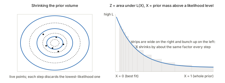
The values L_i are known from the samples. The prior masses X_i are not, but can be estimated without knowing the shape of L:
- Draw N live points from the prior. Their prior masses above their likelihood, sorted, are N uniform numbers on [0,1]: the proportion of the prior with higher likelihood is uniform because we drew from the prior.
- Throw away the worst point (lowest likelihood L_1). Everything above L_1 has mass X_1, which is the largest of N uniforms, and the other N-1 points are uniform on [0,X_1]. The fraction t=X_1/X_0 has density Nt^{N-1} (eq. 73), so \mathbb E[\ln t]=-1/N.
- Replace the discarded point by a new draw from the prior restricted to likelihood above L_1 (typically by a short MCMC run started from one of the survivors). We have N uniform points again, on the smaller region.
- Repeat. After i rounds, \ln X_i\approx-i/N with a spread of about \sqrt i/N.
So the mass shrinks geometrically, by the same factor each round, wherever the likelihood sits. That is why the strips in the picture are wide on the right and narrow near the peak.
import numpy as np

def nested_sampling(log_like, sample_prior, constrained_step, n_live=100, n_iter=1000, rng=None):
    rng = rng or np.random.default_rng()
    live = [sample_prior(rng) for _ in range(n_live)]
    logL = np.array([log_like(x) for x in live])
    log_Z, log_X_prev = -np.inf, 0.0
    for i in range(1, n_iter + 1):
        worst = int(np.argmin(logL))
        log_X = -i / n_live                                    # expected shrinkage
        log_w = np.log(np.exp(log_X_prev) - np.exp(log_X))     # width of the strip
        log_Z = np.logaddexp(log_Z, logL[worst] + log_w)
        log_X_prev = log_X
        keep = rng.integers(n_live)                            # start from a survivor
        live[worst] = constrained_step(live[keep], threshold=logL[worst], rng=rng)
        logL[worst] = log_like(live[worst])
    return log_Z                                               # (plus the remaining live points)
Why it survives phase transitions where tempering does not (Figure 1 of the paper). A tempered posterior at inverse temperature \beta is dominated by the place on the \ln L–\ln X curve where the slope equals -1/\beta-ish: raising \beta moves along the curve by following its slope. Where the curve bends the wrong way (a region where \ln L against \ln X is convex, as at a first-order phase transition), no \beta lands there. The tempered distribution has to jump from one branch to the other and any chain following it gets stuck. Nested sampling walks down the X axis at a steady rate and does not care what shape L(X) has.
The practical cost is the step 3 sampling under a hard constraint L>L_1. The paper lists answers: ellipsoid fits (Mukherjee et al.), clusters of ellipsoids for several peaks (MultiNest, limited to tens of parameters by the clustering), Hamiltonian and Galilean Monte Carlo that bounce off the constraint boundary, “demon” variables that smooth it, and diffusive nested sampling, which fixes the shrinkage per level instead of estimating it.
Example 1: signal detection (section 5.1)
Setting. Decide whether a known waveform s(t) is present in M channels, each coupled by a known weight C_m, with unknown amplitude \alpha>0 and Gaussian noise of known level \sigma_n. Two models (eqs. 74–75): noise only x_m(t)=n_m(t), and signal plus noise x_m(t)=\alpha C_ms(t)+n_m(t).
The odds ratio is Z_{S+N}/Z_N (eq. 76). Divide the signal-plus-noise likelihood by the noise-only one. The parts that depend on x only through x^2 cancel, leaving
\frac{L_{S+N}(\alpha)}{L_N}=\exp\Big\{\frac{\alpha}{\sigma_n^2}\underbrace{\sum_{m,t}C_mx_m(t)s(t)}_{\text{cross-correlation}}-\frac{\alpha^2}{2\sigma_n^2}\sum_{m,t}C_m^2s^2(t)\Big\}.
With a Gaussian prior on \alpha (mean \hat\alpha, standard deviation \sigma_\alpha) and the abbreviations S^2=\sigma_n^2/\sigma_\alpha^2, D=S^2+\sum C_m^2s^2 and E=S^2\hat\alpha+\sum C_mx_ms (eqs. 85–88), the exponent is a quadratic in \alpha. Complete the square, D\alpha^2-2E\alpha+S^2\hat\alpha^2=D(\alpha-E/D)^2-E^2/D+S^2\hat\alpha^2, and the integral over \alpha is a Gaussian integral, giving eq. (90):
\frac{Z_{S+N}}{Z_N}=\exp\Big\{\frac{E^2/D-S^2\hat\alpha^2}{2\sigma_n^2}\Big\}\frac{Z_d}{Z_\alpha}.
If \alpha may take either sign, the two Gaussian normalisers are \sqrt{2\pi\sigma_n^2/D} and \sqrt{2\pi\sigma_\alpha^2} and the log odds ratio is (eq. 98, which I checked and which is right)
\log\mathrm{OR}_\pm=\tfrac12\Big[\frac{E^2}{D\sigma_n^2}-\frac{\hat\alpha^2}{\sigma_\alpha^2}+\log\frac{S^2}{D}\Big].
If \alpha>0 is enforced, the normalisers become half-Gaussians and carry the erf factors of eqs. (93–95). In words: the evidence-based detector is a squared (matched-filter) cross-correlation, plus constants that depend on the prior. That is a satisfying outcome for a derivation: it says the classical correlator is what the Bayesian answer looks like when the prior is not informative, and it names exactly which prior terms the classical one throws away.
A reading to check. In this setup C_m, s(t), \sigma_n and the prior are all fixed, so D is a constant and the only data-dependent quantity in the log odds ratio is the cross-correlation \sum C_mx_ms. Both detectors are then monotone functions of one number (for \mathrm{OR}_\pm, up to the sign symmetry; for \mathrm{OR}_+ the mixture over \alpha>0 of increasing exponentials is increasing in the correlation). Two detectors that are monotone functions of the same statistic have the same ROC curve and the same area under it. The paper reports different areas (Figures 3 and 4), so the “Correlation Method” baseline must be something else, most plausibly a correlation coefficient normalised by the energy of each window, which is a different statistic. The comparison may still be fair, but “beats correlation” then means “beats normalised correlation”, which is a weaker claim than it sounds. The experiment is described in a companion paper [115], not here, and I have not checked it.
Examples 2–4 (sections 5.2–5.4)
Light sensor (5.2). The sensor’s spatial sensitivity is modelled as a mixture of 1 to 4 Gaussians (6 parameters each), and nested sampling estimates each model’s \log Z from calibration sweeps over a black-and-white surface. Table 1 reports \log Z=-665.1\pm2.4 for one Gaussian and -669\pm12 for two, with the three- and four-Gaussian rows far lower and with large uncertainties. The one-Gaussian model has the highest mean evidence and is chosen. The paper itself says the error bars are large enough that “selection of a best model based on the log-evidence alone is not clear”, and blames the degeneracies of mixtures (swapping two components changes nothing, so the likelihood has K! identical peaks and the constrained sampling in step 3 struggles).
Exoplanets (5.3). Four effects add to the light curve of a star with a planet: the planet’s reflected light (Lambertian phases, eq. 101), its thermal emission (day and night sides, eq. 102), Doppler beaming of the star (eq. 103, shifted in phase by \pi/2 against the other two), and the tides the planet raises on the star. Each subset of effects is a theory; MultiNest computes each evidence and the Occam factor automatically discounts effects the data cannot resolve. The point of the example is the framing: “which physical effects are detectable in this data?” is a model-selection question.
Force fields (5.4). Compare molecular-mechanics force fields by the evidence of NMR data they give for a protein, which penalises a force field that fits only by being unconstrained. Same recipe, much larger parameter spaces, where nested sampling and its variants (Hamiltonian, demon variables) are being pushed.
Questions and doubts
Slips in the printed equations (each checked by redoing the algebra):
- Eq. (23), the Laplace variance. \sigma^2=-\big(\tfrac12(\ln p)''\big)^{-1} is twice the value needed. From eq. (22), \ln p\simeq\ln p(x_0)+\tfrac12(\ln p)''(x-x_0)^2, matching -(x-x_0)^2/2\sigma^2 gives \sigma^2=-1/(\ln p)''. As printed, eq. (24) would read -(x-x_0)^2/\sigma^2, not /2\sigma^2.
- Eqs. (29)–(30). Eq. (29) divides by the Z of eq. (30), which includes the factor p(x_0); the Gaussian in (29) does not carry that factor. They are consistent if (29) is read as a density and (30) as the integral of the unnormalised p, but the same symbol means two things.
- Eq. (38), importance sampling for a ratio of evidences. Not the estimator derived in eq. (37); see above.
- Eqs. (60)–(66), notation. The data are written M and the evidence P(M\mid I), though M was the theory everywhere else.
- Eq. (69) and the sentence after (70). F=-\mathrm{KL}+C, not +\mathrm{KL}, and the bound is maximised. The sentence “estimated by minimizing the negative free energy” should say maximising.
- Eq. (7) has the same expression on both sides, and eq. (20) writes D for the data in some places and d in others.
Things that are not slips but deserve care:
- The evidence is sensitive to the prior width, and that is a feature with a catch. Z\propto1/\Delta x for a flat prior. Doubling \Delta x halves the evidence and, if the other theory has no such parameter, halves the odds ratio. So a Bayes factor is only as meaningful as the prior ranges, and a prior wide “to be safe” can swing the answer arbitrarily (Lindley’s paradox). With an improper prior the Occam factor is zero and the evidence is undefined. The paper says priors “must be assigned” but gives little guidance for the case where you have no strong information.
- The paper says nested sampling “elegantly circumvents” the path choice. True of the path; it replaces it with a different problem, sampling inside a hard likelihood contour, which is where all the listed variants (ellipsoids, Hamiltonian, demons, diffusive levels) go to work. In high dimensions that is exactly as hard as before; it is displaced, not removed.
- Table 1 and degeneracy. The error bars grow with model order faster than the means move, which suggests the numbers for three and four components are mostly measuring sampler failure. The choice of one Gaussian is plausible on parsimony grounds, but the gap between one and two (\approx4 in the log, against a standard deviation of \approx12 on the second) is not distinguishable from zero on the paper’s own numbers.
- Variational Bayes underestimates uncertainty under a product-form Q because \mathrm{KL}[Q\,\|\,P] penalises mass where P is small more than missing mass where it is large. The paper treats F as an evidence estimate; a lower bound whose slack you cannot measure (it contains the unknown evidence) cannot tell you how wrong it is.
- Laplace for mixtures. The posterior of a mixture model has K! symmetric peaks; Laplace around one peak misses a factor K! in the evidence unless added by hand, which matters when comparing models with different K.
- “Probability is not decision theory” (the closing remark) is the part most often ignored: the posterior probability of a theory is not the same as a reason to choose it, because costs of wrong choices differ. The paper recommends using the posterior in an expected-utility calculation and leaves it there.
- Is the thermodynamic-integration estimate biased in practice? Eq. (49) is a left-endpoint Riemann sum of a non-decreasing function (the curve in the picture never falls), so it underestimates the integral for any finite number of steps, on top of the Monte-Carlo noise in each average. Whether that or the sampling error dominates depends on the problem.
Takeaways
- The evidence is the probability a theory gave the data, averaged over its own prior; Occam’s razor is that average, not an add-on penalty. Z=L_{\max}\times (fraction of the prior that fits).
- Compare theories by Bayes factors, but remember the prior ranges are inside every evidence, and posterior odds need prior odds too.
- Laplace is “peak height × peak volume”; importance sampling needs tame weights; thermodynamic integration is the area under a never-falling curve of average log-likelihood against \beta; AIS is unbiased where exponentiated thermodynamic integration is biased low; variational Bayes is \log Z=F+\mathrm{KL} with F computable; nested sampling turns a many-dimensional integral into \int_0^1L(X)\,dX with \ln X falling by 1/N per step.
- The detection derivation is clean (completing a square), and the result is a squared matched filter with prior-dependent constants. The claim that it beats plain correlation should be read with the baseline in mind.
- When reading a review like this one, check the formulas: several of the equations above are mis-signed, mis-scaled or mislabelled in the printed version, none fatal, all of the kind that costs an afternoon if copied into code.