MICCAI 2026: domain adaptation and generalisation — the mathematical constructs
Why this page exists
These are the 26 MICCAI 2026 posters and orals tagged domain
adaptation / generalisation that were on arXiv at the time of
reading (from
paper-list-csv/miccai2026-radiology-papers.csv). Each one
gets a short reading of only its core idea and the mathematical
objects it is built from: the score, loss or estimator, what
distribution or divergence it uses, and which known tool it is an
instance of. Results and datasets are left out on purpose. Each entry
ends with What to watch, which names the assumption the maths
leans on or the step that is heuristic rather than derived.
Each entry also has a figure of its core construct. Most are computed from small toy numbers rather than taken from the paper, so they show the mechanism, not the paper’s results. Where a toy exposes a gap in the paper, such as a gate that can never close, the caption says so.
Equations were reconstructed from pdftotext output. Where a paper gives a construct only in words, or its printed equation looks wrong, the entry says so rather than guessing silently.
Construct map
A quick index by the kind of mathematics used. Several papers appear more than once.
| Construct | Papers |
|---|---|
| Mahalanobis / Gaussian feature statistics | MaRS (M-PM-011), PROTON (W-PM-180) |
| EM and latent-variable label noise — see EM | HierEM (M-PM-042) |
| Optimal transport / Wasserstein / Schrödinger bridge — see OT | WALDO (W-AM-013), SC-UNSB (T-PM-095) |
| Flow matching and diffusion priors as input-space adaptation | TTA-Flow (T-AM-049), PET-Adapter (W-PM-054) |
| Entropy minimisation and information maximisation | CoWA (T-PM-200), IMaX (W-PM-007), ReGA (T-AM-061) |
| Uncertainty decomposition and active acquisition | ASFOSDA (T-AM-114), CHILD (W-PM-044), PromptGate (W-AM-192) |
| Prototypes, cosine similarity and relation (Gram) matrices | PSP (M-PM-058), ContiStain (T-AM-027), PROTON (W-PM-180), IntraStyler (T-PM-123) |
| Self-supervised inner loops and test-time training | MedTS-TTT (T-PM-214), VesselSim (W-AM-160), BeatRhythm-TTA (W-PM-078) |
| Variational energies on the output | HD-TTA (W-PM-124) |
| Invariance by construction (augmentation, geometry, pairwise differences) | One Sequence (W-PM-047), CoRe-DA (W-PM-142), JANUS (W-PM-207), EchoTracker2 (T-PM-169), MKGA (M-PM-145) |
| Policy optimisation for VLM reasoning (GRPO) | BrReMark (W-PM-122) |
Interactive figures
The static figures below each freeze one setting of a toy. The interactive page has one widget per paper that lets you move those settings yourself. Each widget runs on small toy numbers in the browser, not on the paper’s data, and each has a callout naming the one thing worth trying. The widgets use their own seeded random draws, so exact values can differ slightly from the static figures while the behaviour matches.
| Widget | What you can do |
|---|---|
| M-PM-011 · MaRS | Drag a test residual around a 2-D residual cloud and compare ‖r‖² with rᵀΣ⁻¹r; then move 16-D OOD energy between the smallest- and largest-λ directions and add a ridge ε the paper lacks, watching AUROC. |
| M-PM-042 · HierEM | Tune a site’s α and β and drag π to see the E-step posterior q; drag raw site sensitivities and change σₐ and the counts to watch the prior shrink them; α = 1 − β collapses q onto π. |
| M-PM-058 · PSP | Rotate, scale, shift and re-start a contour and watch its Fourier descriptor stay fixed; add boundary noise, and meet a phase-scrambled shape with the same descriptor but a different outline. |
| M-PM-145 · MKGA | Change the gate weights, the refinement kernel and the artefact size, and read how much skip energy survives in the nodule versus at the artefacts; raising W_s lets the spikes through. |
| T-AM-027 · ContiStain | Drag tokens, rotate, reflect, add relative drift or shuffle token order, and watch the teacher, student and difference relation matrices and L_rel update. |
| T-AM-049 · TTA-Flow | Change the entry step, speckle and tissue share, and toggle histogram matching; with matching on, the entry step has no effect, because both maps preserve rank order. |
| T-AM-061 · ReGA | Move S_v, λ, S_b, α and λ₁ to see SICE and its floor, and compare the teacher’s memory kernel and half-life with a reference EMA momentum. |
| T-AM-114 · ASFOSDA | Drag target samples on the embedding circle and vary the query budget and the SDD weight; at weight 0 the near-duplicate clump takes two of three queries, at 1 it gets one. |
| T-PM-095 · SC-UNSB | Vary slide drift, texture growth and tile count, and compare per-tile instance norm with the interpolated dense norm, with the seam jump shown live; a “μ̂ only” mode shows σ must be interpolated too. |
| T-PM-123 · IntraStyler | Drag the query, positive and negatives on the style sphere and change τ to read each InfoNCE weight; slide t to compare SLERP with the straight blend, up to where SLERP breaks at 180°. |
| T-PM-169 · EchoTracker2 | Pick window size and stride, scale wall and apical motion, and play the cardiac cycle to see which paths leave the window; a switch compares Euclidean distance with the square-window test. |
| T-PM-200 · CoWA | Set five class probabilities or load samples A–C, rebuild M from simulated predictions, and switch to an off-diagonal-only distance to see that the unit diagonal is what penalises the no-finding sample. |
| T-PM-214 · MedTS-TTT | Drag W₀ in fast-weight space, vary η·λ_max and the number of inner steps, and see Δ = QW₀ − η(QKᵀ)G computed as linear attention. |
| W-AM-013 · WALDO | Drag the projection direction θ and the reference cloud to watch sliced W₂ project, sort and pair; switch the weighting to expose the rank-indexing issue in Eq. 1, and compare DPP, random and nearest-K reference picks. |
| W-AM-160 · VesselSim | Grow a vessel tree with heading noise, branching decay, the branching exponent γ (3 is Murray’s law) and depth; a second toy runs test-time adaptation on L_rec as it drifts away from L_seg. |
| W-AM-192 · PromptGate | Rotate t_OOD or drag any prototype and see the argmax sectors and leaked artefacts against the shared-only boundaries; run an active-learning round and see that softmax temperature never changes the gate. |
| W-PM-007 · IMaX | Move α, imbalance, λ and K to compare the Shannon and Tsallis pushes and the optimal marginal against the true long tail. |
| W-PM-044 · CHILD | Replay a 400-sample stream with the Otsu threshold, the one-sided query band and the budget, and compare errors for the base detector and for CHILD. |
| W-PM-047 · One sequence to segment them all | Pick one of nine label-preserving transforms, set its strength and redraw its parameters, and see how well 300 random draws cover a T2-like or T1-like target; none gets close. |
| W-PM-054 · PET-Adapter | Run 1-D Poisson MLEM while changing iterations, blur, counts and a hidden null-space detail; NLL always falls while RMSE turns back up, and the hidden detail barely moves the measurements. |
| W-PM-078 · BeatRhythm-TTA | Pick a corruption, drag its severity and τ_q, and place 320 toy beats on the reachable 0.067–0.366 SQI band; τ_q = 0.05 gates nothing, and at τ_q ≈ 0.2 clean beats are dropped while muscle noise passes. |
| W-PM-122 · BrReMark | Switch between real, synthetic and healthy scans, edit one response’s IoU, judge and format scores and the gates, and watch the group-standardised advantages; nearly equal rewards still give advantages of about ±1.5. |
| W-PM-124 · HD-TTA | Change the neighbour region’s intensity and texture, toggle the island, and move λ_inf and γ while both energies optimise live and S_rep picks one; a different texture with the same mean is still accepted. |
| W-PM-142 · CoRe-DA | Drag the true target and set the number of exemplars, noise, scale error, offset, absolute-head shift and training pull; the scale error cancels mid-range but biases the edges, and a full pull makes both heads agree on the wrong value. |
| W-PM-180 · PROTON | Change the shift angle, shifted share, gate γ and τ, and read live AUROCs, running variance, α_t and bank contamination; MCM AUROC is 0.00 while α_t stays near 0.6. |
| W-PM-207 · JANUS | Change organ size, gate slope and bias and the sign of the evidence; z_v never changes, the 8-token case is vetoed, and negative evidence lets the gate push p above the visual-only value. |
The papers
M-PM-011 · MaRS: Robust Out-of-Distribution Detection via Mahalanobis Residual Scoring
Francesco Di Salvo, Sebastian Doerrich, Christian Ledig — arXiv:2606.22649
Core idea. OOD detection on frozen foundation-model features, built around the covariance of autoencoder reconstruction residuals. A small autoencoder learns a projection onto the in-distribution (ID) feature manifold. The residual r = z - \hat z is then scored with a Mahalanobis distance instead of \lVert r\rVert_2^2. The residual covariance is highly anisotropic, and OOD deviations concentrate in its low-variance directions, which a uniform \ell_2 norm drowns out.
Mathematical constructs.
- Learned manifold projection. With z = \Phi(x)\in\mathbb{R}^D from a frozen backbone \Phi, an MLP autoencoder (E,D) is trained on ID features with \mathcal{L}_{AE} = \lVert z - \hat z\rVert_2^2, where \hat z = D(E(z)). It is read as a nonlinear projection \Pi_{\mathcal{M}_{ID}}(z) = D(E(z)). This is the nonlinear analogue of the PCA-residual detector.
- Residual covariance. r(x) = z - \Pi_{\mathcal{M}_{ID}}(z) and \Sigma = \operatorname{Cov}(r(x) \mid x\sim \mathrm{ID}), a single global, label-free covariance. Subtracting the projection removes class-semantic variation, which is the paper’s argument for why no class-conditional Gaussians are needed.
- MaRS score (Mahalanobis in residual space). S_{\mathrm{MaRS}}(x) = r(x)^\top \Sigma^{-1} r(x) = \sum_{i=1}^{D} \frac{\big(u_i^\top r(x)\big)^2}{\lambda_i},\qquad \Sigma = U\Lambda U^\top . The spectral form shows the mechanism: each principal residual direction u_i is reweighted by \lambda_i^{-1}, so stable (small-\lambda_i) directions are amplified. The \ell_2 score is the special case \Sigma = I. Residual-PCA is a hard 0/1 version of this weighting.
- Energy ratio diagnostic. \rho_i = \mathbb{E}_{OOD}[(u_i^\top r)^2] / \mathbb{E}_{ID}[(u_i^\top r)^2] is compared between high- and low-variance eigen-subspaces. This is the empirical justification for inverse-variance weighting.
- Decision rule. Threshold S_{\mathrm{MaRS}} at a percentile (e.g. 95th) of ID validation scores.
- Pre-normalisation features. The method is applied before the backbone’s final LayerNorm, because normalisation flattens the eigenvalue spectrum that the score exploits.
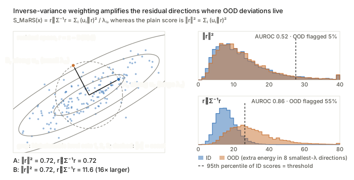
Figure. Points A and B have the same \lVert r\rVert^2, yet r^\top\Sigma^{-1}r is 16 times larger for B because it points along a small-\lambda_i direction, and that reweighting is what separates the OOD histogram on the right.
What to watch. \Sigma^{-1} in D = 384 or 768 dimensions is dominated by the smallest eigenvalues, and the paper states no shrinkage or ridge term, so conditioning is the fragile point. Eq. (4) also uses uncentred r (no residual mean). The Mahalanobis form is only “optimal” under an implicit Gaussian residual model, in which case S\sim\chi^2_D.
M-PM-042 · HierEM: Deep EM with Hierarchical Latent Label Modelling for Multi-Site Prostate Lesion Segmentation
Wen Yan, Yipei Wang, Shiqi Huang et al. — arXiv:2603.14418
Core idea. Each site’s single annotation Y_k is treated as a noisy observation of a latent clean mask G_k, through a class-conditional noise model with site- and case-level sensitivity and specificity. This is STAPLE/Dawid–Skene-style, but with one label per case and “site as reader”. A logistic-normal hierarchical prior partially pools these noise rates towards global means. EM alternates between a voxel-wise posterior over G_k and fitting the CNN to that soft posterior, so the network learns the latent mask rather than a site’s contouring style.
Mathematical constructs.
- Image prior. \pi_k(x) = p_\theta(G_k(x)=1 \mid X_k) = \sigma(f_\theta(X_k)_x).
- Noise model (voxel-independent given G). p(Y=1\mid G=1)=\alpha_{s,k} and p(Y=0\mid G=0)=\beta_{s,k}, i.e. p(Y\mid G;\alpha,\beta) = \begin{cases}\alpha^{Y}(1-\alpha)^{1-Y}, & G=1\\ (1-\beta)^{Y}\beta^{1-Y}, & G=0.\end{cases}
- Hierarchical logistic-normal prior (a GLMM with random effects). \operatorname{logit}\alpha_{s,k} = \mu_\alpha + a_s + u_k and \operatorname{logit}\beta_{s,k} = \mu_\beta + b_s + v_k. The effects have Gaussian priors a_s\sim\mathcal N(0,\sigma_a^2), u_k\sim\mathcal N(0,\sigma_u^2) (similarly b_s, v_k), with sum-to-zero constraints \sum_s a_s = \sum_s b_s = 0. The site-level rates are \alpha_s = \sigma(\mu_\alpha + a_s).
- E-step (Bayes rule per voxel). q_k(x) = \frac{\pi_k(x)\,p(Y_k(x)\mid G=1)}{\pi_k(x)\,p(Y_k(x)\mid G=1) + (1-\pi_k(x))\,p(Y_k(x)\mid G=0)} . For example, Y=1 gives q = \pi\alpha / (\pi\alpha + (1-\pi)(1-\beta)).
- M-step (A). Soft-target CE plus soft Dice: \mathcal L_{seg}(\theta) = \sum_{k,x}\mathrm{CE}(q_k(x),\pi_k(x)) - \sum_k \mathrm{Dice}(q_k,\pi_k).
- M-step (B), binomial-logit MAP from expected sufficient statistics. The statistics are TP_k=\sum_x q_kY_k, P_k=\sum_x q_k, TN_k=\sum_x(1-q_k)(1-Y_k) and N_k=\sum_x(1-q_k). The objective is Q(\phi)=\sum_k\big[TP_k\log\alpha_{s_k,k}+(P_k-TP_k)\log(1-\alpha_{s_k,k})+TN_k\log\beta_{s_k,k}+(N_k-TN_k)\log(1-\beta_{s_k,k})\big], maximised as Q(\phi) - \sum \tfrac{1}{2\sigma^2}(\cdot)^2 with L-BFGS. The \ell_2 penalty is the Gaussian prior acting as shrinkage.
- Uncertainty. Binary predictive entropy H_i = -p_i\log p_i-(1-p_i)\log(1-p_i), evaluated through risk–coverage \mathrm{Risk}(c) = 1-\mathrm{Dice}(S_c).
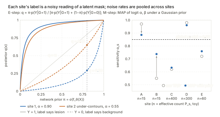
Figure. The dashed Y=0 curves show that a low site sensitivity \alpha_s lets the network prior \pi override a missing label, and the right panel shows the Gaussian prior on \operatorname{logit}\alpha_s pulling data-poor sites towards \sigma(\mu).
What to watch. With one label per case, (\pi,\alpha,\beta) are only weakly identifiable. The case effects u_k, v_k are pinned down mainly by the prior, and the E-step’s prior is the network’s own output, which risks self-confirmation. Stability relies on initialisation (\mu\approx\operatorname{logit}0.9) and a decaying auxiliary loss on the observed labels.
M-PM-058 · PSP: Harnessing Position and Shape Priors for Cross-Domain Few-Shot Medical Image Segmentation
Bin Xu, Yazhou Zhu, Haofeng Zhang — arXiv:2606.28799 (arXiv v1; v2 withdrawn)
Core idea. Cross-modality few-shot prototype segmentation, built on quantities assumed to be modality-invariant: organ position and contour shape. Relative polar coordinates are injected into the features. A support prototype is reweighted channel-wise by its agreement with an explicit shape descriptor (signed-distance statistics plus invariant Fourier descriptors). The prototype is then calibrated towards the query distribution before cosine-similarity prediction.
Mathematical constructs.
- Polar position embedding. With image-centred coordinates (\bar h,\bar w): \rho_{h,w}=\sqrt{\bar h^2+\bar w^2} and \theta_{h,w}=\operatorname{arctan2}(\bar w,\bar h). An MLP lifts these to F_p, and a gated residual gives \hat F = (1-\beta)F + \beta\,\mathrm{SA}\big(\mathrm{CM}([F, F_p])\big), where \beta is learnable (initialised to 0.1).
- Geometric statistics. From the signed distance map of M_s, the max, mean and variance over the foreground form v_{geo}\in\mathbb R^3.
- Fourier shape descriptors. Boundary points become complex signals z_m = x_m + i y_m, with DFT coefficients Z_u. The descriptor is v_{spec}(i) = \frac{\lvert Z_{i+1}\rvert}{\lvert Z_1\rvert},\quad i=0,\dots,N_{spec}-1 . Dropping Z_0 gives translation invariance, dividing by \lvert Z_1\rvert gives scale invariance, and taking magnitudes gives rotation and start-point invariance. Only low frequencies are kept (N_{spec}=15). Then P_{prior}=\mathrm{MLP}([v_{geo}, v_{spec}])\in\mathbb R^{C_s}.
- Shape-prior channel attention. F_{seq} = \mathrm{MLP}(\mathrm{Flatten}(\mathrm{AAP}(\hat F_s\odot M_s)))\in\mathbb R^{C\times C_s}, and w_i = \mathrm{ReLU}\!\left(\frac{F_{seq}^{(i)}\cdot P_{prior}}{\lVert F_{seq}^{(i)}\rVert_2\lVert P_{prior}\rVert_2}\right),\qquad P_s' = \mathrm{MAP}(\hat F_s, M_s)\odot w .
- Hybrid prototype. A coarse map \tilde M_q^{coar} = \cos(\hat F_q, P_s') gives P_q=\mathrm{MAP}(\hat F_q,\tilde M_q^{coar}), and P^* = P_s' + \mathrm{CA}(P_s', P_q, P_q). The prediction is \tilde M_q = 1-\sigma\big(-\alpha(\cos(\hat F_q, P^*) - \tau)\big) = \sigma\big(\alpha(\cos-\tau)\big), with \alpha=20 and a learned threshold \tau=\mathrm{FC}(\hat F_q).
- Loss. Pixel BCE on the query plus the PANet-style reverse alignment loss (query to support): \mathcal L = \mathcal L_{prim}+\mathcal L_{align}.
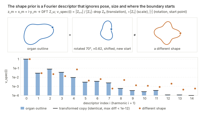
Figure. The black ticks from the rotated, rescaled, shifted and re-started contour sit exactly on the blue bars of v_{spec}(i)=\lvert Z_{i+1}\rvert/\lvert Z_1\rvert, while a genuinely different shape (orange) does not.
What to watch. “Position invariance” presumes support and query share a field of view and centring. Magnitude-only Fourier descriptors discard phase, so distinct shapes can collide. The text calls the attention weight a sigmoid probability while Eq. (6) uses ReLU. The invariance claims are heuristic and not formalised.
M-PM-145 · MKGA: Multi-Kernel Gated Decoder Adapters for Robust Multi-Task Thyroid Ultrasound under Cross-Center Shift
Maziar Sabouri, Nourhan Bayasi, Arman Rahmim — arXiv:2603.08906
Core idea. An architectural rather than probabilistic method. The object is the skip connection of a multi-task U-Net-style decoder. Skip features are refined with two receptive fields and then multiplied by a context-conditioned attention gate before fusion, so artefact-prone shallow content (speckle, calipers, text) is suppressed. The claimed benefit under shift is reduced negative transfer between geometry-driven segmentation and texture-driven TI-RADS classification.
Mathematical constructs.
- Multi-kernel refinement. X^{ref}_{skip} = \phi_{1\times1}\big(\mathrm{Conv}_{3\times3}(X_{skip}) \,\Vert\, \mathrm{Conv}_{3\times3,d=2}(X_{skip})\big), where the dilated branch has an effective 5\times5 receptive field and \Vert is channel concatenation.
- Additive attention gate (Attention U-Net form). \alpha = \sigma\Big(\psi\big(\delta(W_g X_{high} + W_s X^{ref}_{skip})\big)\Big),\qquad X^{gate}_{skip} = \alpha\odot X^{ref}_{skip}, where W_g, W_s, \psi are 1\times1 convolutions, \delta is ReLU, and X_{high} is the upsampled deeper decoder feature.
- Residual fusion. Y_{MKGA} = F_{res}(X_{high}\,\Vert\,X^{gate}_{skip}), with two conv–norm–ReLU blocks.
- ResMKGA bottleneck correction. X^{enh}_{high} = F_{enc} + \mathrm{SE}(\phi_{3\times3}(F_{enc})). This is a residual squeeze-and-excitation channel recalibration.
- Multi-task objective. \mathcal L = \mathcal L_{Dice}+\mathcal L_{CE}^{pixel} + \lambda_{mal}\mathcal L_{mal} + \lambda_{pos}\mathcal L_{pos}.
- Optional gradient surgery (PCGrad, standard rule; not written out in the paper). If g_i^\top g_j<0, then g_i \leftarrow g_i - \frac{g_i^\top g_j}{\lVert g_j\rVert^2} g_j, which projects out the conflicting component on the shared encoder. For MedSAM, LoRA uses W = W_0 + BA with rank r\in\{4,16,32\}.
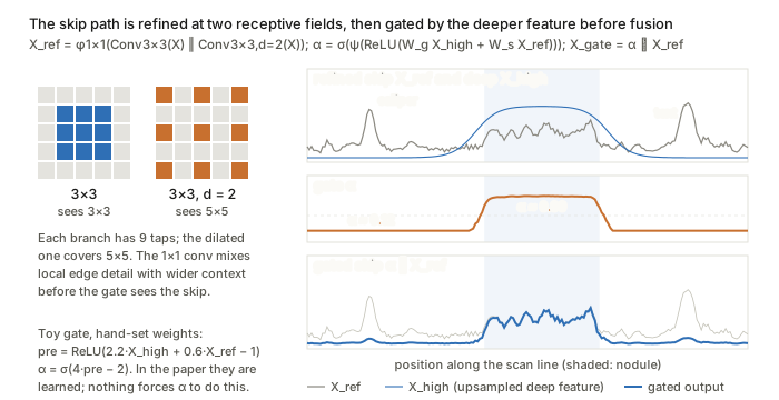
Figure. The gate \alpha=\sigma(\psi(\mathrm{ReLU}(W_gX_{high}+W_sX^{ref}_{skip}))) is driven by the smooth deep feature, so it passes nodule texture and damps the caliper and text spikes; the weights here are hand-set, not learned.
What to watch. No shift model, bound or invariance is stated. The robustness argument is qualitative: gating is assumed to down-weight artefact regions, but nothing constrains \alpha to do so rather than to fit source-centre cues.
T-AM-027 · ContiStain: Cross-Domain Relation-Preserving Distillation for Continual Multi-Domain Virtual IHC Staining
Fuqiang Chen, Yifeng Wang, Hongpeng Wang et al. — arXiv:2607.03851
Core idea. Continual learning over sequentially arriving stain domains (biomarkers). The object preserved is not the outputs or the weights but the cross-domain token-level cosine-similarity (Gram) matrix between the generator’s renderings of old biomarkers from the same H&E input. The matrix is measured in a domain-aware mixture-of-experts feature space. Keeping this relational geometry fixed against a frozen teacher limits forgetting while leaving the student free to adapt to the new domain.
Mathematical constructs.
- Domain conditioning by FiLM at the bottleneck. h_b' = (1+\gamma_b(d))\odot h_b + \beta_b(d), where [\gamma_b,\beta_b]=\phi_b(u_d) and u_d=\psi(e_d) embeds a one-hot domain code.
- Domain- and content-routed MoE. For sampled and projected tokens z_{\ell,d}=\phi_\ell(\mathrm{Sample}(f_{\ell,d})): w_\ell = \mathrm{softmax}\big(g_\ell([z_{\ell,d},u_d])\big),\qquad F_{\ell,d} = \mathrm{Normalize}\Big(\sum_{m=1}^{M} w_{\ell,m}\odot h_{\ell,m}(z_{\ell,d})\Big).
- Routing regulariser. \mathcal L_{MoE} = \lambda_1\,\mathrm{BCE}(w_{\ell,m^\star}, y_d) + \lambda_2\Big(\max_m \bar p_m - \tfrac1M\textstyle\sum_m \bar p_m\Big). The first term ties domain d to a reference expert m^\star. The second is a load-balancing penalty on the mini-batch mean routing probabilities \bar p_m.
- Cross-domain relation matrix. For old domains i,j and teacher or student (\cdot)\in\{t-1,t\}, applied to generated images \tilde y_i^{(\cdot)} = G_{(\cdot)}(x,i): R_\ell^{(\cdot)}(i,j) = \mathrm{Normalize}(F^{(\cdot)}_{\ell,i})\,\mathrm{Normalize}(F^{(\cdot)}_{\ell,j})^\top\in\mathbb R^{P\times P}.
- Relational distillation (RKD-style). \mathcal L_{rel} = \frac{1}{\lvert\mathcal P\rvert\lvert\mathcal S\rvert}\sum_{(i,j)\in\mathcal P}\sum_{\ell\in\mathcal S}\big\lVert R^t_\ell(i,j) - R^{t-1}_\ell(i,j)\big\rVert_1 . For the second domain, where only one old domain exists, output-level \ell_1 distillation is used instead.
- Total loss. \mathcal L = \mathcal L_{base}^{ASP} + \lambda_{rel}\mathcal L_{rel} + \lambda_{moe}\mathcal L_{MoE}. Here \mathcal L_{base}^{ASP} is the adversarial plus patch-contrastive loss on the current domain.
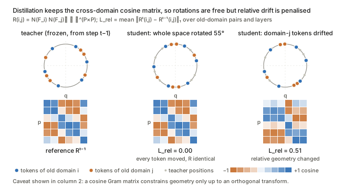
Figure. Rotating the whole feature space leaves R_\ell(i,j) and \mathcal L_{rel} at zero, and only drift of one domain relative to the other is penalised, which shows both how the loss works and its invariance to orthogonal transforms.
What to watch. A cosine Gram matrix is invariant to orthogonal transforms of the feature space, so it constrains geometry only up to rotation. It also needs identical token-sampling positions across i, j, teacher and student. The link between preserved relations and preserved output quality is argued, not proven.
T-AM-049 · TTA-Flow: Test-Time Adaptation in Optical Coherence Tomography Using Trajectory-Aligned Time-Independent Flow
Veit Hucke, Thomas Pinetz, Gregor Reiter et al. — arXiv:2606.18876
Core idea. Input-space test-time adaptation. A flow-matching generative model trained only on the high-SNR source device treats a noisy low-cost scan as an intermediate point on a generation trajectory and integrates the remaining ODE to a source-like surrogate. Two devices bridge the gap between real noise and the ideal Gaussian path. First, histogram matching maps the test image’s intensity distribution to the average marginal of simulated trajectories at a chosen step. Second, the velocity network is not time-conditioned, so it infers the effective noise level itself.
Mathematical constructs.
- Flow ODE and continuity equation. \frac{dz_t}{dt} = v_t(z_t) with z_0\sim\mathcal N(0,I), inducing p_t with \partial_t p_t + \nabla\cdot(p_t v_t)=0.
- Linear (rectified-flow / conditional-OT) path. z_t = (1-t)z_0 + t y, with target velocity u_t = y - z_0 and \mathcal L_{FM} = \mathbb E_{t,z_0,y}\big\lVert v_\theta(z_t) - (y - z_0)\big\rVert_2^2 . This is deterministic, with no Ornstein–Uhlenbeck forward noising.
- x-prediction parameterisation. The network predicts x_\theta(z_t)\approx y, and the velocity is recovered as v_\theta(z_t) = \frac{x_\theta(z_t) - z_t}{1-t}. The network takes no t input (“noise-unconditional”), following He et al.
- Euler sampling. z_{i+1} = z_i + \tfrac1S v_\theta(z_i), with S=100.
- Reference trajectory marginals. Simulate n trajectories and average the per-step intensity histograms to obtain \{\bar H_s\}_{s=1}^S.
- Histogram matching as 1-D optimal transport. z_{s_{target}} = F_{\bar H_{s_{target}}}^{-1}\circ F_\zeta(\zeta), the monotone rearrangement (the W_2-optimal map between intensity marginals). The ODE is then integrated from s_{target} to S, SDEdit-style, with no data-fidelity term. The step s_{target} is a grid-searched hyperparameter.
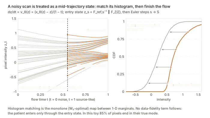
Figure. The quantile map F^{-1}_{\bar H_{s}}\circ F_\zeta on the right places the noisy pixels on the s_{target} marginal, and from there the source-trained ODE (orange, left) carries them to the source modes with no further tie to the input.
What to watch. Matching only the first-order intensity marginal ignores spatially correlated speckle. Without data fidelity, the only tie to the patient is the initial state, so lesions can be hallucinated or erased. The Euler step still uses the schedule’s t through 1/(1-t). The prose writes \zeta\approx t z + (1-t)y, which inverts the convention of Eq. (2).
T-AM-061 · ReGA: Test-time Adaptation of Pelvic Bone Segmentation Models via Dynamic Reliability-Guided
Ling Ren, Chao Deng, Ziming Wang et al. — arXiv:2608.00510
Core idea. Online teacher–student TTA driven by a scalar per-sample reliability score (SICE). SICE is built from MC-dropout agreement in both region overlap (soft Dice) and boundary distance (percentile Hausdorff), and is calibrated by normalised predictive entropy. The score then gates everything else: feature-bank admission and fusion, centroid weighting in a contrastive loss, the loss weight and the EMA rate. Unreliable pseudo-labels therefore contribute less under domain shift.
Mathematical constructs.
- Volumetric consistency (soft Dice against K dropout passes). S(x,\hat x) = \frac{1}{KL}\sum_{k=1}^{K}\sum_{l=0}^{L-1}\frac{2\sum_{v}x^l_v\hat x^l_{k,v}}{\sum_v x^l_v + \sum_v \hat x^l_{k,v}},\qquad S_v = S(P_i,\hat P_{ik}).
- Boundary discrepancy. This is a symmetric \gamma-percentile Hausdorff distance on Canny edges: S_b = \max\{P_\gamma(B_i,\hat B_{ik}), P_\gamma(\hat B_{ik}, B_i)\}.
- Reliability and entropy calibration. R_i = \lambda_1 S_v + \lambda_2 e^{-S_b/\alpha} and \lambda = 1 - \frac{1}{\lvert\Omega\rvert\log C}\sum_{v}\Big(-\sum_l \bar P_{v,l}\log\bar P_{v,l}\Big),\qquad \mathrm{SICE}_i = \lambda R_i, where \bar P is the dropout-ensemble mean.
- Trust-weighted feature refinement. A FIFO bank admits Z_i when \mathrm{SICE}_i exceeds the running \tau-percentile. With Z_f=\sum_j W_j Z_j and W_j = \mathrm{sim}(Z_i,Z_j)/\sum_j\mathrm{sim}(Z_i,Z_j), the refined feature is Z_i' = w(\mathrm{SICE}_i)Z_i + (1-w(\mathrm{SICE}_i))Z_f.
- Confidence-weighted centroids and contrastive loss. c_l = \frac{\sum_j f_j(Z_i)\,\mathbf 1(\hat y_j=l)(1-E_i)\,\mathrm{SICE}_i(l)}{\sum_j\mathbf 1(\hat y_j=l)} and \mathcal L_{rc} = -\frac1L\sum_l\log\frac{\exp(\mathrm{sim}(c_l,c_l))}{\sum_{m\ne l}\exp(\mathrm{sim}(c_l,c_m))}, with temperature-scaled cosine similarity.
- Reliability-adaptive mean teacher. \phi_{t+1} = (1-\mathrm{SICE}_i)\phi_t + \mathrm{SICE}_i\,\theta_{t+1} and \mathcal L = \frac1B\sum_i\big(\mathcal L_m(p_i'',p_i) + \mathrm{SICE}_i\,\mathcal L_{re}(p_i',p_i) + \beta\mathcal L_{rc}\big).
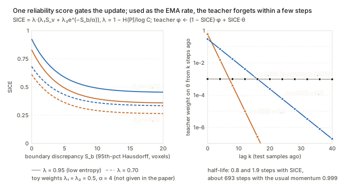
Figure. SICE falls with boundary disagreement S_b and scales with the entropy factor \lambda; used directly as the EMA step, it gives the teacher a memory half-life of 1–2 samples, against about 693 samples at momentum 0.999.
What to watch. As written, the numerator of \mathcal L_{rc} is the constant \exp(1/T), so the loss reduces to a pure inter-class repulsion (log-sum-exp) term. Using SICE directly as the EMA step gives far faster teacher drift than the usual momentum of about 0.999. SICE measures dropout self-consistency, which is a proxy for accuracy and not a calibrated error estimate.
T-AM-114 · ASFOSDA: Active Source-free Domain Adaptation in Open-set Medical Image Segmentation via Decomposed Uncertainty and Prototype Discrepancy
Jin Yang, Yichi Zhang, Peijie Qiu et al. — arXiv:2606.08749
Core idea. An active-learning acquisition score for source-free, open-set adaptation: the target label set has C_t > C_s classes, and the unknown classes \mathcal{C}_u = \mathcal{C}_t \setminus \mathcal{C}_s are what the score looks at. The score combines two things computed over test-time augmentations (TTA) of each unlabelled volume: an uncertainty term (mean entropy plus the variance of the free energy) and a feature-space diversity term (cosine distance to “source-like” prototypes and to other candidates). The idea is to spend the annotation budget on target samples that are uncertain, far from what the source model already handles, and not redundant with one another.
Mathematical constructs.
- Class-aware aleatoric uncertainty (CAU): mean entropy under TTA. Let p^{j}_i be the probability map of unknown class i for augmentation j (j=0 is the original), with m augmentations. Then \mathrm{CAU}(x_u) = \frac{1}{1+m}\sum_{j=0}^{m}\Big(-\sum_{i=1}^{t-s} p^{j}_i \log p^{j}_i\Big). This is the “expected entropy” half of the usual entropy decomposition, but the average is over input perturbations, not over a parameter posterior.
- Class-aware epistemic uncertainty (CEU): variance of free energy. Using logits z^{j}_i of the unknown classes and temperature T=1, E(x^{j}_u) = -T\log\sum_{i=1}^{t-s} e^{z^{j}_i/T},\qquad \mathrm{CEU}(x_u)=\frac{1}{1+m}\sum_{j=0}^{m}\big(E(x^{j}_u)-\bar E\big)^2, where \bar E is the mean energy over the 1+m views. The free energy is the energy-based OOD score (Liu et al. 2020), and CEU is its empirical variance under TTA.
- Decomposed score. \mathrm{CDU}=\mathrm{Norm}(\mathrm{CAU})+\mathrm{Norm}(\mathrm{CEU}), where Norm is min–max scaling followed by a uniform quantile transform, so that the two terms share a common scale.
- Class-agnostic prototype discrepancy (CPD). Take encoder embeddings L^1,\dots,L^K of the K lowest-CDU samples as source-knowledge prototypes, and H^1,\dots,H^K of the K highest-CDU samples as candidates. Then \mathrm{CPD}(x_u)=\underbrace{\frac1K\sum_{j=1}^{K}\Big(1-\tfrac{H^u\cdot L^j}{\lVert H^u\rVert\,\lVert L^j\rVert}\Big)}_{\text{cross-domain (CDD)}}+\underbrace{\frac{1}{K-1}\sum_{i\neq u}\Big(1-\tfrac{H^u\cdot H^i}{\lVert H^u\rVert\,\lVert H^i\rVert}\Big)}_{\text{self-domain (SDD)}}. CDD rewards distance from the source-like samples, and SDD is a diversity term similar to a core-set criterion.
- Target-refined self-training. First fit \mathcal{L}_{\text{sup}} on the queried set \mathcal{T}_l. The resulting target-trained model then regenerates pseudo-labels for \mathcal{T}_u, and training continues on \mathcal{L}=\mathcal{L}_{\text{sup}}(Y^l,P^l)+\mathcal{L}_{\text{unsup}}(Y^u,P^u).
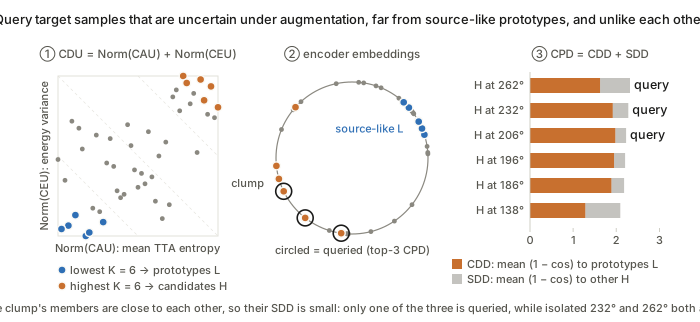
Figure. Uncertainty (\mathrm{CDU}) picks the candidates; then the self-domain term of \mathrm{CPD}=\mathrm{CDD}+\mathrm{SDD} stops the query budget from being spent on the three near-duplicate candidates in the clump. The toy assumes the top-\mathrm{CPD} candidates are queried; the paper only says high-scoring samples are selected.
What to watch. The “epistemic” term is variance under input augmentation, not uncertainty over parameters, so it is not a Bayesian epistemic measure. The entropy and energy are also computed on unknown-class output channels, which the source model never saw labels for. How voxel-wise maps are reduced to one score per volume is not spelled out.
T-PM-095 · SC-UNSB + dual-level KD: Two-Stage Cross-Domain Cervical Abnormality Screening with Cytopathological Image Synthesis and Knowledge Distillation
Jincheng Li, Yuzhi He, Yihui Zhan et al. — arXiv:2606.27678
Core idea. Stage 1 builds a synthetic intermediate domain by translating source images with a Schrödinger bridge, i.e. entropy-regularised optimal transport between the source and target image distributions. It is modified so that normalisation statistics vary smoothly with pixel position, which removes tiling seams in gigapixel slides. Stage 2 distils a source-side detector into a target-side detector by matching feature distributions (MMD) at two depths. The shallow depth uses low-pass-filtered features and the deep depth uses a projected semantic embedding.
Mathematical constructs.
- Schrödinger bridge (from UNSB). Find the path measure closest in KL to Brownian motion that has the prescribed endpoint marginals: \min_{\mathbb{Q}}\ \mathrm{KL}(\mathbb{Q}\,\Vert\,\mathbb{W})\quad \text{s.t.}\quad \mathbb{Q}_0=\pi_0,\ \mathbb{Q}_1=\pi_1, where \mathbb{W} is the Wiener measure. Its static form is entropic OT with quadratic cost. UNSB approximates it with a discrete-time Markov chain trained adversarially.
- Dense (spatially continuous) normalisation. Plain instance norm \gamma\,(x^{(k)}-\mu^{(k)})/\sigma^{(k)}+\beta uses one set of statistics per patch k, which causes discontinuities at patch boundaries \partial\Omega_k. SC-UNSB replaces these with fields obtained by bilinear interpolation over the 3\times3 patch neighbourhood \mathcal{N}_k: \hat\mu(p)=\Phi_{\text{interp}}\big(\{\mu^{(n)}\}_{n\in\mathcal N_k},p\big),\quad \hat\sigma(p)=\Phi_{\text{interp}}\big(\{\sigma^{(n)}\}_{n\in\mathcal N_k},p\big), G_{\text{SC}}(x^{(k)},t)=\mathrm{Conv}\Big(\gamma\odot\frac{x^{(k)}-\hat\mu(p)}{\hat\sigma(p)}+\beta\Big).
- Feature alignment loss. A mean-embedding (linear-kernel) MMD plus a reconstruction anchor: \mathcal L_{\text{MMD}}=\Big\lVert \tfrac1B\textstyle\sum_{i}\phi(\hat F_S^i)-\tfrac1B\sum_j\phi(\hat F_T^j)\Big\rVert_2^2,\qquad \mathcal L_{\text{MSE}}=\lVert F_S-\hat F_S\rVert_2^2. The printed equation omits the second 1/B, which is presumably a typo.
- Loose alignment (LFA, shallow layers). Source side: a multi-scale low-pass filter \hat F_S=\Phi(\mathrm{AvgPool}_{k_a\times k_a}(F_S)) with bilinear upsampling \Phi. Target side: a learnable version, \hat F_T=\mathrm{Conv}_{3\times3}(\mathrm{Concat}[\mathrm{Down}(F_T),\mathrm{MSLF}(F_T)]). Compact alignment (CFA) applies the same losses after a 1\times1 projection of penultimate features into a shared space Z.
- Objective. \mathcal L=\mathcal L_{\text{cls}}+\mathcal L_{\text{loc}}+\alpha(\mathcal L_{\text{LFA}}+\mathcal L_{\text{CFA}}). The student is also supervised by teacher pseudo-labels with confidence above 0.9.
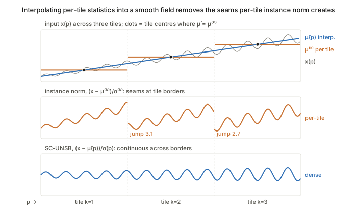
Figure. Compare the middle and bottom strips: per-tile statistics \mu^{(k)},\sigma^{(k)} create jumps of about 3 units at tile borders, and the interpolated fields \hat\mu(p),\hat\sigma(p) remove them.
What to watch. The claim that dense normalisation “constrains the bridge to spatially continuous functions” is intuition, not something the paper proves. The KL objective is only reached through UNSB’s adversarial surrogate. Linear-kernel MMD matches only first moments in \phi-space. The “frequency-domain” filter is spatial average pooling, not a Fourier operation.
T-PM-123 · IntraStyler: Intra-Domain Style Synthesis for Cross-Modality MRI Domain Adaptation
Han Liu, Yubo Fan, Hao Li et al. — arXiv:2601.00212
Core idea. The target domain (T2 MRI) is treated as a continuum of styles rather than a single distribution or a few labelled sub-domains. A 3D style encoder learns unit-norm style vectors on the hypersphere through contrastive learning, with negatives that share anatomy but not style. Those vectors then condition an unpaired translator through adaptive instance normalisation. Any target image can therefore serve as a style reference, so synthetic source-to-target data covers the scanner and protocol variability within the target domain.
Mathematical constructs.
- Anatomy-invariant InfoNCE. Query y and positive y^+ are two crops of the same image, so they share style but differ in anatomy. Negatives are intensity-perturbed positives, y^-_n=\epsilon_n(y^+), drawn from contrast change, Gaussian smoothing, noise, bias field, or a mix; they share anatomy with the positive but differ in style. The embeddings v,v^+,v^-_n\in\mathbb{S}^{K-1} are \ell_2-normalised, and the loss is an (N{+}1)-way cross-entropy: \mathcal L_{\text{style}}=-\log\frac{\exp(v\cdot v^+/\tau)}{\exp(v\cdot v^+/\tau)+\sum_{n=1}^{N}\exp(v\cdot v^-_n/\tau)},\qquad \tau=0.01.
- Dynamic instance normalisation (AdaIN-type conditioning). Normalise z_{\text{norm}}=(z-\mu)/\sigma per channel, then apply z_{\text{out}}=\gamma_v\,z_{\text{norm}}+\beta_v. Here (\gamma_v,\beta_v) come from a 1\times1\times1 convolution of the style vector v=E_S(y), and these layers replace the last two IN layers of the decoder.
- Style consistency (cycle in embedding space). \mathcal L_{\text{con}}=-\,E_S(y)\cdot E_S(G(x)), the negative cosine similarity between the reference style and the style of the translated source image.
- Joint objective. The CUT/QS-Attn losses plus the two style terms, trained end to end: \mathcal L=\mathcal L_{\text{adv}}+\lambda_{\text{NCE}}\mathcal L_{\text{PatchNCE}}+\lambda_{\text{style}}\mathcal L_{\text{style}}+\lambda_{\text{con}}\mathcal L_{\text{con}}. PatchNCE is the patch-wise InfoNCE of CUT between input and output patches, which preserves content.
- SLERP style interpolation. Interpolation follows the geodesic on the sphere, so the norm stays at 1: \mathrm{SLERP}(v_0,v_1;t)=\frac{\sin((1-t)\theta)}{\sin\theta}v_0+\frac{\sin(t\theta)}{\sin\theta}v_1,\qquad \theta=\arccos(v_0\cdot v_1).
- Reference selection. References are chosen by K-means on the style embeddings, with the number of clusters picked by silhouette score, taking one representative image per cluster.
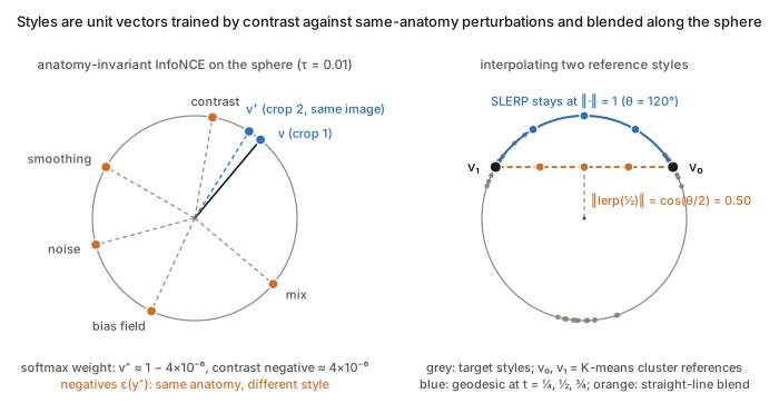
Figure. With \tau=0.01, even a negative 30° away gets softmax weight of about 4\times10^{-6}; on the right, SLERP stays on the sphere while the linear blend’s midpoint shrinks to \cos(\theta/2)=0.5.
What to watch. “Style” is defined operationally by the perturbation family \epsilon. The encoder is therefore invariant to anatomy only relative to those synthetic transforms, and the positive pair assumes style is spatially stationary within a volume. Pooling to a single global vector cannot represent local style variation.
T-PM-169 · EchoTracker2: Enhancing Myocardial Point Tracking by Modeling Local Motion
Md Abulkalam Azad, Vegard Holmstrøm, John Nyberg et al. — arXiv:2605.12140
Core idea. Myocardial motion is continuous and bounded from frame to frame, so the tracker drops the global coarse-initialisation stage of general point trackers and searches correspondences only in a local window. Robustness to shifts in view or anatomy comes from this inductive bias, not from an explicit adaptation objective. Three pieces make it work: temporally mixed features at every scale, local 4D correlation volumes, and attention over each point’s K nearest neighbouring trajectories.
Mathematical constructs.
- Problem. Given a video V\in\mathbb{R}^{T\times H\times W\times C} and queries \{(x_i^{t_q},y_i^{t_q})\}_{i<N}, estimate the trajectories \mathcal T=\{(x_i^t,y_i^t)\} over one cardiac cycle.
- iTSM-ResNet. A temporal shift module (TSM: shift some channels by \pm1 frame) is inserted after each ResNet block, not only the last: F^{(\ell+1)}=\begin{cases}\mathrm{TSM}_\ell\big(B_\ell(F^{(\ell)})\big), & \ell\in\{0,1,2\}\\ B_\ell(F^{(\ell)}), & \ell=3\end{cases} This gives every scale local temporal context, with a receptive field of 7 frames at the deepest block.
- Local 4D correlation. Query features Q^{(\ell)}\in\mathbb{R}^{N\times r\times r\times d} are sampled in an r\times r window around each query, and frame features F^{(\ell)}_c\in\mathbb{R}^{T\times N\times r\times r\times d} in a window around the current trajectory estimate. All-pairs cosine similarity gives C^{(\ell)}_{t,n,u,v,u',v'}=\cos\big(Q^{(\ell)}_{n,u,v},\,F^{(\ell)}_{c;t,n,u',v'}\big)\in\mathbb{R}^{T\times N\times r\times r\times r\times r}, which is encoded to D dimensions and concatenated over three scales (r=9 chosen by ablation). This is the LocoTrack-style 4D correlation, and the bounded-displacement prior enters through the window size r.
- KNP-Joint transformer and iterative refinement. Multi-head self-attention runs along time and across each point’s K nearest trajectories (K=10), which encodes a spatial-coherence prior. It predicts residuals, \mathcal T^{(m)}=\mathcal T^{(m-1)}+(\Delta x,\Delta y)^{(m)}, over 4 iterations.
- Loss. \mathcal L=\frac1m\sum_{i=1}^{m}\gamma^{m-i}\,\mathrm{L1}(\mathcal T^{(i)},\mathcal T^{\text{gt}}) with \gamma=0.8, the RAFT-style exponentially weighted sequence loss.
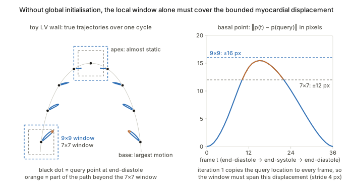
Figure. In the first iteration the query location is copied to every frame, so the r\times r window has to cover the whole end-systolic excursion; in this toy only r=9 does, in line with the paper’s ablation.
What to watch. Everything rests on inter-frame displacement staying inside the correlation window at feature stride. Low frame rates or large apical motion would violate this. The paper contains no explicit domain-adaptation construct, so its out-of-distribution claims are empirical.
T-PM-200 · CoWA: Leveraging Pathology Co-occurrence for Test-Time Adaptation in Chest X-Ray Diagnosis
Woojin Jeong, Yujin Choi, Dongbin Kim et al. — arXiv:2607.03715
Core idea. This is TENT-style entropy minimisation for multi-label classification, with a weight on each sample. The weight measures how well the sample’s predicted label configuration agrees with a label co-occurrence matrix estimated online from the model’s own target predictions. Samples whose predicted pathology pairs are implausible under that structure are down-weighted. This reduces noisy gradients, which would otherwise reinforce confident but incoherent predictions under shift.
Mathematical constructs.
- Online co-occurrence estimate. Binarise the predictions \hat y_i=f_\theta(x_i)\in[0,1]^C at a fixed threshold to get \tilde y_i\in\{0,1\}^C. Accumulate over all batches seen so far: S=\sum_{i=1}^{n}\tilde y_i\tilde y_i^{\top},\qquad P=S/n,\qquad M_{jk}=\frac{P_{jk}}{\sqrt{P_{jj}P_{kk}}+\varepsilon},\ \ M_{jj}=1. M is the Ochiai (cosine) coefficient between the label-indicator columns, a correlation-like normalisation of joint frequencies. Because S is cumulative, early noisy predictions get diluted over time.
- Consistency weight (Gaussian kernel in Frobenius distance). With the soft outer product m_i=\hat y_i\hat y_i^{\top}, w_i=\exp\!\Big(-\frac{\lVert m_i-M\rVert_F^2}{\tau}\Big). An ablation favours the Frobenius norm over \ell_1, \ell_2 and \ell_\infty, because it aggregates squared deviations over all entries.
- Weighted entropy objective. With floor w_{\min}=0.01, \mathcal L_{\text{CoWA}}=\frac1B\sum_{i=1}^{B}\max(w_i,w_{\min})\,H(\hat y_i), where only the BatchNorm affine parameters are updated, as in TENT. For multi-label outputs, H is presumably the sum of per-class binary entropies.
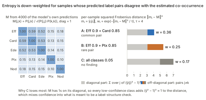
Figure. A and B differ only in which pair they predict, so the off-diagonal part of \lVert m_i-M\rVert_F^2 is what separates w=0.36 from 0.25; the no-finding sample C gets the lowest weight because of the diagonal (\hat y^2-1)^2 terms, which is the unit-diagonal issue raised under What to watch.
What to watch. m_i is an unnormalised soft outer product, while M is normalised with unit diagonal. The distance therefore mixes structural mismatch with confidence: diagonal terms (\hat y_{ij}^2-1)^2 penalise any low-probability class. M is also estimated from the very predictions being adapted, so a biased early estimate can reinforce itself; the paper offers no bound on this.
T-PM-214 · MedTS-TTT: Test-Time Training for Medical Time Series Classification
Mingzhi Chen, Yiyu Gui, Guibo Luo — arXiv:2606.21329
Core idea. Adaptation to subject-level shift is built into each layer as a fast-weight linear map. For each sample, the map takes one gradient step on a self-supervised regression from keys to the residual V-K, and the updated map is then applied to the queries. This is a TTT-layer construction (Sun et al.): the inner loop is a single closed-form SGD step, and the slow weights are meta-learned by the supervised outer loss. The same computation runs at train and test time, so adaptation needs no labels and no iterative optimisation.
Mathematical constructs.
- Tokeniser. A channel-wise temporal convolution gives U=\phi(F_t(X)). A spatial convolution over channels gives S=\phi(F_s(U))\in\mathbb{R}^{B\times D\times T}. Patch projection with stride P and a learned positional embedding gives \tilde H=\mathcal P(S)+PE_{[:L]}, with L=\lceil T/P\rceil.
- Self-supervised inner objective. With multi-head projections Q,K,V and fast weights W_{\text{fast}}, Z=KW_{\text{fast}},\qquad \mathcal L_{\text{TTT}}=\tfrac12\big\lVert \mathrm{LN}(Z)-(V-K)\big\rVert_2^2 .
- One-step fast-weight update. With G=\partial\mathcal L_{\text{TTT}}/\partial Z, W_{\text{fast}}\leftarrow W_{\text{fast}}-\eta\,K^{\top}G,\qquad \Delta=QW_{\text{fast}}, where \eta is a head-wise adaptive step size. K^{\top}G is exactly \partial\mathcal L_{\text{TTT}}/\partial W_{\text{fast}}, so \Delta=QW_0-\eta\,QK^{\top}G. In this form the layer is equivalent to a linear-attention-like update in which G plays the role of values.
- Gated convolutional backbone. First [A,R]=HW_{\text{in}}. Then the main branch passes through a depthwise short conv and the TTT module, \tilde A=\mathcal M(\phi(F_{dw}(A))). The layer output is \Delta H=\big(\phi(R)\odot\tilde A\big)W_{\text{out}},\qquad H^{(k+1)}=H^{(k)}+\Delta H^{(k)}, a GLU-style multiplicative gate on a residual stream.
- Training. The outer cross-entropy \mathcal L_{\text{CE}} updates only the slow parameters, differentiating through the inner step. At test time only the label-free inner step runs.
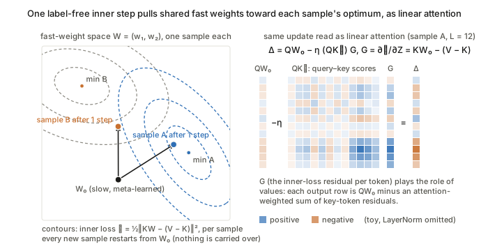
Figure. One label-free step W_0-\eta K^{\top}G moves each sample’s fast weights toward that sample’s own minimum and is reset for the next sample; equivalently \Delta=QW_0-\eta(QK^{\top})G is linear attention with the inner-loss residuals G as values (LayerNorm omitted in the toy).
What to watch. The update is per sample and is not carried over between samples, so this “test-time training” is a data-dependent layer rather than persistent adaptation. Nothing forces the V-K reconstruction target to align with the shift that matters for classification; any benefit comes from meta-learning, and the paper gives no guarantee.
W-AM-013 · WALDO: Wasserstein-Aligned Localisation for VLM-Based Distributional OOD Detection in Medical Imaging
Bernhard Kainz, Johanna P. Mueller, Matthew M. G. Baugh et al. — arXiv:2605.05161
Core idea. Zero-shot VLM anomaly localisation is recast as comparative inference: the query is shown next to healthy references, and the choice of references is made with optimal transport. Each image becomes an empirical distribution of DINOv2 patch tokens, and references are ranked by an entropy-weighted sliced Wasserstein distance between those distributions. The method is training-free. It adapts to a new domain only through which in-distribution references it retrieves.
Mathematical constructs.
- Patch distributions. An image x maps to the point cloud P_x=\{\phi_1,\dots,\phi_T\}\subset\mathbb{R}^{768} with T=(H/16)(W/16). Comparing these as empirical measures keeps spatial and textural structure that a single CLS vector would collapse.
- Sliced Wasserstein. Exact W_2 between two T-point clouds costs O(T^3) as a linear programme, so it is replaced by SW_2^2(P,Q)=\mathbb{E}_{\theta\sim\mathcal{U}(\mathbb{S}^{d-1})}\big[W_2^2(\theta^\top P,\theta^\top Q)\big],\qquad W_2^2(P_\theta,Q_\theta)=\tfrac1T\textstyle\sum_{i=1}^T (p_{(i)}-q_{(i)})^2, where p_{(i)},q_{(i)} are sorted 1-D projections. Monte-Carlo with M directions gives cost O(TM\log T).
- Entropy weighting. Each patch gets weight w_i=H(\phi_i)/\sum_j H(\phi_j), where H(\phi)=-\sum_k\sigma_k(\phi)\log\sigma_k(\phi) and \sigma is a softmax over feature channels. This gives SW_2^{(w)}(P,Q)=\Big(\textstyle\sum_{i=1}^T w_i\,(p_{(i)}-q_{(i)})^2\Big)^{1/2}.
- “Goldilocks” bias–variance argument. With reference distance d(q,h), the localisation error is decomposed as \mathbb{E}[\epsilon^2]=\mathrm{Bias}^2(d)+\mathrm{Var}(d). Bias falls as d\to0 (anatomy matches) and variance rises (differences sit near the VLM’s discrimination threshold); the reverse holds as d\to\infty. References are therefore drawn from the [\alpha,1-\alpha] percentile band of SW_2^{(w)}, with \alpha=0.3.
- DPP-style diversity. The selected set is H^*=\arg\max_{\lvert S\rvert=K}\det(L_S), where L_{ij}=q_iq_j\exp(-\beta\,SW_2(h_i,h_j)) and q_i=\mathbb{1}[h_i\in\text{zone}]. This is a quality-gated similarity kernel, so the determinant rewards references that are spread out.
- Self-consistency aggregation. Boxes from the K references are merged by NMS with discounted confidences \tilde c_k^{(j)}=c_k^{(j)}\exp(-\lambda\,SW_2(P_q,P_{h_k})).
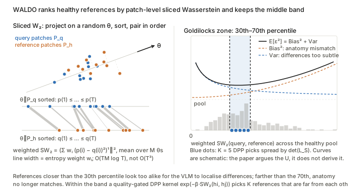
Figure. Left, SW_2 only needs sorting of 1-D projections, with w_i as line width; right, references are drawn from the [\alpha,1-\alpha]=[0.3,0.7] percentile band where the argued (not derived) \mathrm{Bias}^2+\mathrm{Var} is lowest, and the DPP spreads the K picks across it.
What to watch. The bias–variance decomposition is a qualitative argument; the paper does not derive \mathrm{Bias}(d) or \mathrm{Var}(d), and the inverted U is observed rather than proved. In Eq. (1) the patch weights w_i are indexed by sorted projection order rather than by patch, and the expectation over \theta is left implicit, so the weighting is heuristic rather than a true weighted-measure OT distance.
W-AM-160 · VesselSim: learning 3D blood vessel segmentation without expert annotations
Erin Rainville, Melissa Ananian, Tristan Mirolla et al. — arXiv:2605.26277
Core idea. The segmenter never sees a real label. It learns vessel geometry from a stochastic procedural model of branching tubular trees, painted with domain-randomised intensities. The remaining synthetic-to-real appearance gap is closed at test time. A self-supervised masked-reconstruction head supplies a label-free loss, and only the encoder’s instance-normalisation affine parameters are updated. The idea is that shift is mostly in first- and second-order feature statistics, while tubular shape is invariant.
Mathematical constructs.
- Stochastic tree generator. This is recursive branching (extending VascuSynth) with a biased random walk for each segment. The heading is updated by a rotation, d_{s+1}=R(a_s,\theta_s)\,d_s, with rotation axis a_s, magnitude \theta_s and segment length sampled from literature-derived ranges. This gives directional persistence with controllable tortuosity. Branching probability decays with depth, growth is breadth-first, and collision checks can terminate a branch.
- Murray’s law for radii. Daughter radii follow physiological scaling, r_{\text{parent}}^3=r_1^3+r_2^3.
- Domain randomisation. Masks are rendered into angiography-like volumes with random 3-D background shapes, Gaussian noise and ellipsoidal “skull” shells (following the VesselFM scheme). The label map stays fixed while the intensity nuisance varies.
- Composite objective. \mathcal{L}_{\text{total}}=\alpha\mathcal{L}_{CE}+\beta\mathcal{L}_{Dice}+\gamma\mathcal{L}_{cbDice}+\lambda\mathcal{L}_{rec},\quad(\alpha,\beta,\gamma,\lambda)=(0.1,0.9,0.2,0.1). \mathcal{L}_{cbDice} is the centreline-boundary Dice, which uses soft skeletonisation (iterated soft min/max-pooling) to compare predicted and true centrelines and boundaries. It is a differentiable topology prior. \mathcal{L}_{rec} is an in-painting loss for a decoder on the shared bottleneck, applied to inputs with random cubes (2^3 to 16^3 voxels) set to -1.
- Test-time adaptation. On unlabelled target patches, minimise \mathcal{L}_{rec} over the instance-norm parameters \{\gamma_\ell,\beta_\ell\} only, where \mathrm{IN}(h)=\gamma\,(h-\mu)/\sigma+\beta. Everything else is frozen. This is test-time training with an auxiliary task learnt jointly during training.
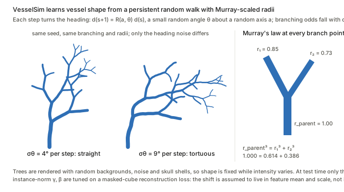
Figure. The per-step rotation noise \sigma_\theta alone sets tortuosity, while r_{\text{parent}}^3=r_1^3+r_2^3 fixes every radius, so geometry is fully procedural and only the intensity rendering is randomised.
What to watch. TTA helps only to the extent that the reconstruction gradient is aligned with the segmentation gradient. Nothing guarantees this; joint training merely encourages it. The generator’s parameter ranges are hand-set, so coverage of real vessel calibres, such as large arteries, is an assumption and not learnt.
W-AM-192 · PromptGate: Client-Adaptive Vision–Language Gating for Open-Set Federated Active Learning
Adea Nesturi, David Dueñas Gaviria, Jiajun Zeng et al. — arXiv:2603.07163
Core idea. A frozen BiomedCLIP acts as a zero-shot (C+1)-way classifier, with C in-distribution classes plus one “OOD” class, to filter each client’s unlabelled pool before any active-learning acquisition. The text side is adapted with CoOp-style learnable context tokens. These are split into a federated (FedAvg) global part and a private per-client part, so the ID/OOD boundary tracks each site’s own artefact distribution without sharing images.
Mathematical constructs.
- Class-specific context (CSC) prompts. For c\in\{1,\dots,C,\text{OOD}\} there are global tokens p_c^g\in\mathbb{R}^{d_p\times D} and client-k tokens p_c^k\in\mathbb{R}^{d_p\times D}, giving t_c^k=E_{\text{text}}\big([p_c^g;p_c^k],\,T_c\big)\in\mathbb{R}^D.
- Cosine-softmax pseudo-labelling. With image embedding z(x)=E_{\text{img}}(x), s_c^k(x)=\frac{z(x)^\top t_c^k}{\lVert z(x)\rVert\,\lVert t_c^k\rVert},\qquad p_c^k(x)\propto\exp\!\big(s_c^k(x)/\tau_{\text{VLM}}\big),\qquad \hat y^k(x)=\arg\max_c p_c^k(x).
- Gate. The candidate pool is C_k^{(r)}=\{x\in U_k^{(r)}:\hat y^k(x)\in\{1,\dots,C\}\}, and any acquisition rule then picks Q_k^{(r)}=\mathcal{A}(C_k^{(r)},L_k^{(r)},\theta_k^{(r)}). The gate is an argmax, so no OOD score threshold is involved.
- Prompt loss. On oracle-labelled queries, \mathcal{L}^{(r)}_{\text{prompt},k}(\phi^g,\phi^k)=\frac{1}{\lvert Q_k^{(r)}\rvert}\sum_{x\in Q_k^{(r)}}\ell_{CE}\big(p^k(x),y(x)\big), with \phi^g=\{p_c^g\}_c and \phi^k=\{p_c^k\}_c.
- Federated split. Only \phi^g updates go to the server, which averages them with FedAvg; \phi^k never leaves the client. This is a partial-personalisation scheme with shared and private parameter blocks.
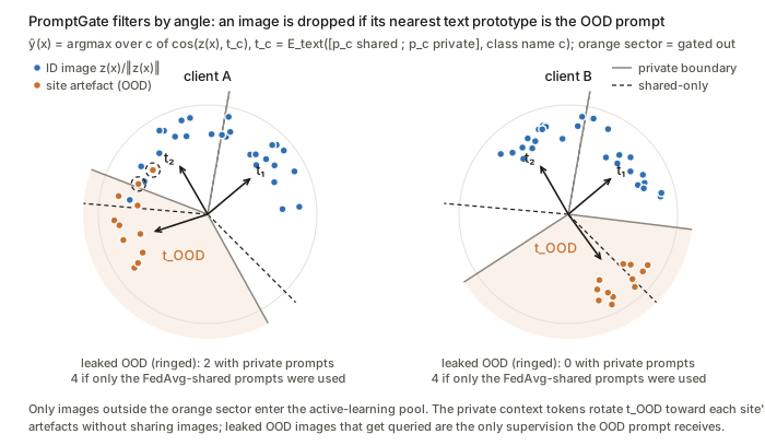
Figure. Because \hat y=\arg\max_c \cos(z,t_c^k) is a nearest-direction rule, the gate is a set of angular sectors, and the private tokens p_c^k rotate t_{\text{OOD}}^k toward each site’s artefacts (solid vs dashed boundaries; geometry hand-set for illustration).
What to watch. Queries come only from the gated pool, so the “OOD” prompt is supervised only by OOD samples that leaked through the gate. It therefore learns from hard false positives, and its early rounds depend on a good zero-shot prior. OOD is modelled as a single class prototype, which assumes that one text direction can cover a heterogeneous set of artefacts.
W-PM-007 · IMaX: Information Maximization for Long-Tailed Semi-Supervised Domain Generalization
Leo Fillioux, Omprakash Chakraborty, Quentin Gopée et al. — arXiv:2603.08434
Core idea. The method is the InfoMax objective I(Y;X)=H(Y)-H(Y\mid X), made semi-supervised by imposing label constraints on the labelled set, with the conditional-entropy term swapped for FixMatch-style pseudo-label cross-entropy. The key change is the marginal-entropy term. Shannon H(Y) equals \log K-D_{KL}(\pi\,\lVert\,u_K) and so pulls predictions towards class balance, which hurts under long tails. It is replaced by a Tsallis \alpha-entropy, which penalises departure from uniform more weakly.
Mathematical constructs.
- Constrained MI. \max_\theta H(Y)-H(Y\mid X) subject to y_i=p_i for all x_i\in D_L. The marginal is estimated as \pi_k\approx\frac{1}{\lvert D\rvert}\sum_{i\in D}p_{ik} over labelled and unlabelled samples. Substituting the constraints gives \min_\theta\sum_k\pi_k\log\pi_k-\frac{1}{\lvert D_L\rvert}\sum_{i\in D_L}\sum_k y_{ik}\log p_{ik}-\frac{1}{\lvert D_U\rvert}\sum_{i\in D_U}\sum_k p_{ik}\log p_{ik}.
- Pseudo cross-entropy in place of H(Y\mid X_U). Weak-view pseudo-labels \hat y_i=\arg\max p_i supervise the strong view p_i^A=f_\theta(A(x_i)): H(\hat Y\mid X_U)=-\frac{1}{\lvert D_U\rvert}\sum_{i\in D_U}\sum_k\mathbb{1}[\max p_i\ge\tau]\,\hat y_{ik}\log p^A_{ik}. This avoids the collapse to a single class that direct conditional-entropy minimisation can cause.
- Tsallis \alpha-entropy. Writing H(Y) as a KL divergence to the uniform distribution and generalising to the \alpha-divergence gives H_\alpha(p)=\log_\alpha K-K^{1-\alpha}D_\alpha(p\,\lVert\,u_K)=\frac{1}{\alpha-1}\Big(1-\sum_k p_k^\alpha\Big), which recovers Shannon entropy as \alpha\to1. For \alpha>1 the entropy surface is flatter near the uniform point, so imbalanced marginals cost less.
- Final objective. \min_\theta\,-H_\alpha(Y)+H(Y\mid X_L)+H(\hat Y\mid X_U). Labelled cross-entropy acts as a penalty that enforces the equality constraints.
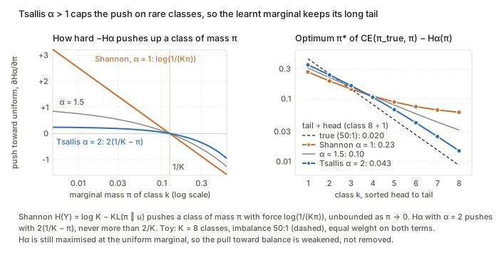
Figure. Shannon’s push on a class, \log(1/(K\pi_k)), diverges as \pi_k\to0, whereas H_\alpha with \alpha=2 pushes with 2(1/K-\pi_k)\le 2/K, so the learnt marginal keeps much more of the long tail.
What to watch. H_\alpha is still maximised at the uniform distribution, so the bias towards balance is softened but not removed, and \alpha is tuned per dataset. The setting assumes that P_Y is shared across domains and that only P_X shifts; the MI view says nothing about domain invariance as such.
W-PM-044 · CHILD: Human-in-the-Loop OOD Detection for Safe Clinical Deployment
Jinlun Ye, Kaiyue Lu, Runhe Lai et al. — arXiv:2609.07188
Core idea. This is training-free, online correction of any scalar OOD score using a small physician-feedback budget. Queries go to a data-adaptive, asymmetric uncertainty band on the 1-D score axis, located by Otsu thresholding of the stream’s score history. The feedback is stored as ID/OOD feature caches, and later scores are shifted by nearest-neighbour cosine similarity, a retrieval-based calibration with no parameter updates.
Mathematical constructs.
- Budgeted streaming decision. The base rule is G(x_t)=\text{ID} if s_t\ge\lambda, else OOD. Queries q_t\in\{0,1\} must satisfy \sum_{t=1}^T q_t\le B=\lfloor\rho T\rfloor, and each decision uses only past observations, so the procedure is causal.
- Otsu boundary. On the history H_t=\{s_i\}_{i\le t}, \tau_t=\arg\max_\tau\sigma_b^2(\tau),\qquad \sigma_b^2(\tau)=\omega_0(\tau)\,\omega_1(\tau)\,\big(\mu_0(\tau)-\mu_1(\tau)\big)^2, where \omega and \mu are the mass and mean of the two groups either side of \tau. This is a 1-D two-class variance split.
- Asymmetric risk interval. The width is \Delta_t=Q_\alpha(H_t)-\min(H_t), a robust low-tail spread with \alpha near 0, and the interval is I_t=[\tau_t,\tau_t+\Delta_t]. It extends only towards the ID side, because OOD-accepted-as-ID is the costly error.
- Cache similarities. For features \phi(\cdot), S_{ID}(x_t)=\max_{\phi(x)\in C_{ID}}\cos(\phi(x_t),\phi(x)), and S_{OOD} is defined in the same way. The soft term is \delta_t=S_{ID}-S_{OOD}.
- Gated hard assignment. Let y_t=\mathrm{sign}(S_{ID}-S_{OOD}) and h_t=\mathbb{1}[\max\{S_{ID},S_{OOD}\}\ge\eta], with H_t=h_ty_t (the paper reuses the symbol H_t). The calibrated score is S_{\text{final}}=s_t+\beta\,(\delta_t+H_t). This is a 1-nearest-neighbour vote from each cache, added to the detector score.
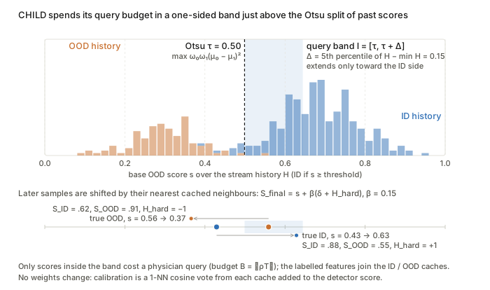
Figure. The query band I_t=[\tau_t,\tau_t+\Delta_t] sits only on the ID side of the Otsu split, and later scores move by \beta(\delta_t+H_t) toward whichever feature cache is nearer.
What to watch. Otsu assumes that the score histogram is roughly bimodal, with ID above OOD. \beta must match the base detector’s score scale, so the additive fusion is not scale-invariant. The width \Delta_t is tied to the minimum score, which makes it sensitive to outliers early in the stream.
W-PM-047 · One Sequence to Segment Them All: Efficient Data Augmentation for CT and MRI Cross-Domain 3D Spine Segmentation
Nathan Molinier, Hendrik Möller, Thomas Dagonneau et al. — arXiv:2605.03098
Core idea. Across CT and MRI sequences the anatomy y is fixed and only the intensity map x=g(y) changes. Single-source domain generalisation is therefore attacked by sampling random label-preserving intensity and texture transforms x\mapsto T(x), in the hope that the family \{T\} covers the unseen contrast mappings. The augmentations are geometric first, then the new appearance transforms, then the default nnU-Net ones, and they run on GPU. The paper is empirical: its “maths” is the transform family itself.
Mathematical constructs.
- Intensity inversion. T(x)=\max x+\min x-x, a min–max range flip that turns bright bone into dark bone (for example CT to T2-like).
- Edge and texture operators. Scharr gradient magnitude \lVert\nabla_S x\rVert with Scharr derivative kernels. Unsharp masking T(x)=x+\lambda\,(x-G_\sigma*x). RandomConv T(x)=k*x with a randomly sampled 3-D kernel k. Each of these swaps absolute intensity for structure that is more contrast-invariant.
- Histogram equalisation. T(x)=\hat F(x), where \hat F is the normalised empirical CDF of voxel intensities. This is the monotone map to an approximately uniform histogram.
- RedistributeSeg (label-conditioned). For each segmented region r, a randomly scaled estimate of that region’s intensity density \hat p_r is added, so T(x)_v=x_v+a_r\,\hat p_r(x_v) for v\in r with random a_r (reconstructed from the paper’s one-line description). This produces region-wise intensity shifts that mimic tissue-specific contrast changes.
- Bias field and random function. A smooth multiplicative inhomogeneity field, and T(x)=f(x) for a randomly drawn nonlinear f.
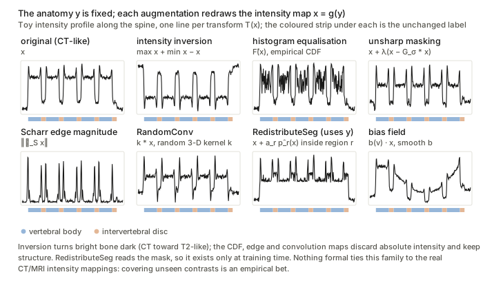
Figure. Every T redraws the intensity map x=g(y) while the label strip y stays identical, and only RedistributeSeg needs the mask, so it can be used only at training time.
What to watch. Nothing formal ties the transform family to the true CT/MRI intensity mappings, so coverage is an empirical hope. RedistributeSeg also uses the ground-truth mask, which makes it a label-dependent augmentation that is not available at test time.
W-PM-054 · PET-Adapter: Test-Time Domain Adaptation for Full and Limited-Angle PET Image Reconstruction
Rüveyda Yilmaz, Yuli Wu, Johannes Stegmaier et al. — arXiv:2605.08030
Core idea. A score-based diffusion prior trained only on phantoms is used inside a MAP reconstruction under the Poisson likelihood. It is adapted to clinical data at dataset level without ground truth. Only MR-conditioned low-rank adapters (conditional LoRA with FiLM modulation) are trained, and the loss is measurement Poisson NLL plus an MR-edge-weighted total-variation term. Sampling is warm-started by diffusion inversion of an OSEM image, which cuts the number of steps from 50 to 2.
Mathematical constructs.
- Forward model. y\sim\mathrm{Poisson}(Ax+b), with system matrix A\in\mathbb{R}^{m\times n}, activity x\ge0 and expected scatter plus randoms b.
- Generalised DDIM/VP-SDE step. x_{t_{k-1}}=\gamma_{t_{k-1}}\hat x_0(x_{t_k})-v_{t_k}\sqrt{v_{t_{k-1}}^2-\eta_{t_k}^2}\;s_\theta(x_{t_k},t_k)+\eta_{t_k}z, with Tweedie’s estimate \hat x_0(x_t)=(x_t+v_t^2 s_\theta(x_t,t))/\gamma_t. Here \eta interpolates between deterministic DDIM and the stochastic SDE, and s_\theta is trained by denoising score matching.
- Data consistency. \hat x_0 is refined into \hat x_{\text{MAP}} by preconditioned gradient ascent on the penalised Poisson log-likelihood, using the EM preconditioner x/(A^\top\mathbf{1}) (following PET-DDS).
- Conditional LoRA. For layer \ell, h_\ell=W_0x_\ell+U\,\phi\big(Dx_\ell\mid g(x_{MR})\big),\qquad \phi(z\mid c)=\gamma_\phi(c)\odot z+\beta_\phi(c), with frozen W_0, D\in\mathbb{R}^{r\times k}, U\in\mathbb{R}^{d\times r} and r\ll\min(d,k). The low-rank update is FiLM-modulated by MR features.
- Adaptation loss. \mathcal{L}_{\text{adapt}}=\mathcal{L}_p+\lambda\mathcal{L}_a. \mathcal{L}_p is the Poisson NLL between y and \hat y=A\hat x_{\text{MAP}}+b, that is \sum_i\hat y_i-y_i\log\hat y_i, with missing-angle bins masked. \mathcal{L}_a is a TV penalty on the reconstruction with MR-derived weights w_j=\exp(-\lVert(\nabla x_{MR})_j\rVert/\sigma): it smooths strongly inside homogeneous tissue and lightly across MR edges, a Bowsher/anisotropic-TV-style anatomical prior.
- Warm start. OSEM/MLEM recovers low-frequency components (large singular values of A) first, the semi-convergence property. The OSEM image is therefore inverted by DDIM to t_r=0.4, and T=2 prior/data-consistency iterations run from there instead of from \mathcal{N}(0,I).
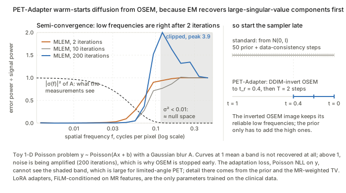
Figure. EM gets the large-singular-value (low-frequency) bands right within 2 iterations, which justifies inverting OSEM to t_r=0.4 and running T=2 steps; the shaded band where \sigma^2<0.01 is what the Poisson NLL cannot constrain.
What to watch. The claim that the OSEM image lies “near the clean-image manifold” is a spectral heuristic, not a bound. Measurement-only adaptation cannot constrain the null space of A, which is large in the limited-angle case, so the anatomy that fills it comes from the MR-weighted TV term. That makes the method’s output depend on PET–MR structural agreement. The prior is also a 2-D slice model used in 3-D.
W-PM-078 · BeatRhythm-TTA: Test-Time Adaptation for ECG Classification via SQI-Gated Self-Training and Beat-Rhythm Consistency
Wenhan Jiang, Zhipeng Deng, Jiale Zhou et al. — arXiv:2608.23347
Core idea. Test-time adaptation of a source ECG classifier is treated as mean-teacher self-training on the BatchNorm affine parameters, with a hard gate on each update. The gate multiplies a teacher-confidence test by an unsupervised, hand-built signal quality index (SQI), so artefact-corrupted segments never produce a gradient. Two cosine-consistency regularisers, one on whole-segment features (“rhythm”) and one on R-peak-centred beat embeddings (“beat”), keep the representation stable under augmentation while the BN statistics drift towards the target.
Mathematical constructs.
- TTA objective. With a classifier f(\cdot;\theta):\mathbb{R}^{C\times T}\to\mathbb{R}^K (multi-label, K diseases), adaptation solves \theta_T=\arg\min_\theta \mathbb{E}_{x\sim\mathcal{D}_T}\,\mathcal{L}_{\text{tta}}(f(x;\theta),x), updating only the BN (\gamma,\beta). There are three protocols: offline, continual online (\theta_i\to\theta_{i+1}) and independent online (reset to \theta_S for every sample).
- Beat SQI as a soft AND. For each beat window x^{(i)}, whose length is scaled by the median RR interval, \mathrm{SQI}^{(i)}=\sigma\big(\mathrm{conc}^{(i)}\big)\,\sigma\big(\mathrm{sharp}^{(i)}\big)\,\sigma\big(-\mathrm{bwr}^{(i)}\big), where conc is the energy ratio of the central QRS region to the window, sharp is a high quantile of \lvert\Delta x\rvert normalised by the RMS, and bwr is the energy ratio of a moving-average baseline to the window. The sample weight is w=\frac{1}{M_b}\sum_i \mathrm{SQI}^{(i)}.
- Gated soft pseudo-labelling. With clean view x_c=x, a time-aligned augmentation \tilde{x}=A(x) and p_\theta=\sigma(f_\theta): \mathcal{L}_{\text{pl}}=\mathbb{1}[c(x)\ge\tau_c]\;\mathbb{1}[w(x)\ge\tau_q]\;\ell_{\text{bce}}\big(p_\theta(\tilde{x}),\,p_{\bar\theta}(x_c)\big),\qquad c(x)=\min_k \big\lvert p_{\bar\theta}(x_c)_k-\tfrac12\big\rvert . Here c is the worst-case per-label margin from 0.5. The teacher is an EMA of the student, \bar\theta\leftarrow\mu\bar\theta+(1-\mu)\theta (mean teacher).
- Rhythm consistency. This is an asymmetric stop-gradient cosine loss, as in BYOL and SimSiam: \mathcal{L}_{\text{rhythm}}=1-\cos\big(\mathrm{sg}(F_c),F_a\big), where F_c=F(x_c) and F_a=F(\tilde{x}) are intermediate features.
- SQI-weighted beat consistency. Beat embeddings b_c^{(i)},b_a^{(i)} are pooled from the features around each R-peak. Then \mathcal{L}_{\text{beat}}=\frac{\sum_i \omega^{(i)}\big(1-\cos(\mathrm{sg}(b_c^{(i)}),b_a^{(i)})\big)}{\sum_i\omega^{(i)}+\epsilon},\qquad \omega^{(i)}=\max\big(\mathrm{SQI}^{(i)},\tau_{\text{floor}}\big), which is a self-normalised, quality-weighted average over beats.
- Total loss. \mathcal{L}=\mathcal{L}_{\text{pl}}+\lambda_{\text{beat}}\mathcal{L}_{\text{beat}}+\lambda_{\text{rhythm}}\mathcal{L}_{\text{rhythm}}.
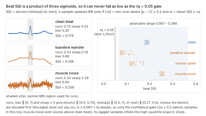
Figure. Compare the shaded attainable range of \mathrm{SQI}=\sigma(\mathrm{conc})\,\sigma(\mathrm{sharp})\,\sigma(-\mathrm{bwr})\in[0.067,0.366] with the dashed \tau_q=0.05 line: taken literally, the quality gate never closes. In this toy, muscle noise also scores above clean beats.
What to watch. The SQI is a heuristic product of sigmoids of raw morphology ratios, with no calibration or probabilistic reading. Everything also depends on R-peak detection staying reliable under the shift. The confidence gate adapts only on target samples the teacher is already sure about, which is a selection bias towards the “easy” part of the target distribution.
W-PM-122 · BrReMark: Enhancing Brain MRI Anomaly Detection and Reasoning with ROI Rethink and Synthetic Data
Shangkun Li, Jie Xu, Yi Guo et al. — arXiv:2606.25894
Core idea. Diagnosis is modelled as a two-turn policy \pi_\theta of a vision-language model. The first turn emits a hypothesis and a bounding box. The box is rendered back onto the image, and the second turn conditions on that marked image to verify the finding and answer. The policy is trained by factorised maximum likelihood (SFT) and then by GRPO with a gated composite reward. Robustness to out-of-distribution (OOD) pathology comes from domain-randomised synthesis: real lesion masks are injected into SynthSeg label maps and rendered with randomised intensities. These synthetic images feed only the localisation part of the RL reward.
Mathematical constructs.
- Two-turn factorisation. o_1=(h,b)\sim\pi_\theta(\cdot\mid I,q), where b=\varnothing for normal scans. Then I_m=\mathrm{render}(I,b) and o_2=(v,y)\sim\pi_\theta(\cdot\mid I,q,o_1,I_m). The SFT loss is the matching chain-rule negative log-likelihood: \mathcal{L}_{\text{SFT}}=-\log\pi_\theta(o_1\mid I,q)-\log\pi_\theta(o_2\mid I,q,o_1,I_m).
- Composite, gated reward. r_i=r_{\text{fmt}}+r_{\text{loc}}+r_{\text{llm}}, with r_{\text{fmt}}\in[0,0.4] (tag completeness), r_{\text{loc}}=\min(\mathrm{IoU},0.5) (a saturating IoU reward) and r_{\text{llm}}\in[0,1] from an LLM judge. Three gates apply. r_{\text{llm}}=0 if the MRI sequence is misidentified. r_i=0 if a lesion is boxed on a healthy scan, a hard false-positive penalty. r_{\text{llm}} is dropped for synthetic samples.
- GRPO objective. The advantage is normalised within a group of G sampled responses, \hat{A}_i=(r_i-\mu_r)/\sigma_r, which removes the need for a value critic: J_{\text{GRPO}}(\theta)=\mathbb{E}\Big[\tfrac{1}{G}\textstyle\sum_{i=1}^G\min\big(\rho_i\hat{A}_i,\ \mathrm{clip}(\rho_i,1-\epsilon,1+\epsilon)\hat{A}_i\big)-\beta\,D_{\mathrm{KL}}(\pi_\theta\,\Vert\,\pi_{\text{ref}})\Big]. The paper writes \rho_i=\pi_\theta(o_i\mid I,q)/\pi_{\text{ref}}(o_i\mid I,q) with \pi_{\text{ref}} the SFT model. Standard PPO and GRPO use \pi_{\text{old}} in the ratio and keep \pi_{\text{ref}} only for the KL term.
- Label-space pathology injection. A real lesion mask is implanted into a healthy SynthSeg label map L to give L'. The implantation site is sampled with weights from a Euclidean distance transform over internal brain tissue, which biases sites towards deep regions so the lesion stays inside the parenchyma.
- Domain-randomised rendering. SynthSeg’s label-conditioned generative model renders L' with random per-label intensities. The lesion intensity prior is truncated to a robust interval, median \pm\,2\timesMAD of real lesions, for example \mu\in[88,195] for T1 tumour.
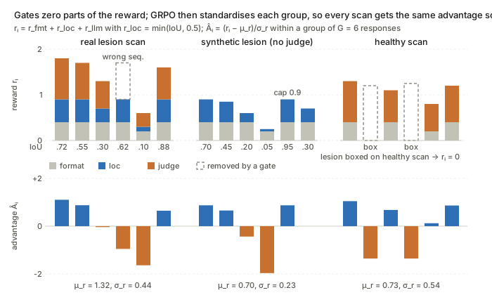
Figure. The dashed boxes show what each gate removes, and the bottom row shows that \hat A_i=(r_i-\mu_r)/\sigma_r gives the synthetic group, capped at 0.9, the same spread of advantages as the real scans.
What to watch. The OOD claim rests on domain randomisation, not on any bound. The reward is hand-tuned, with caps and gates, and partly delegated to an LLM judge, so the policy optimises a proxy objective. The exact form of the distance-transform sampling density is not given.
W-PM-124 · HD-TTA: Hypothesis-Driven Test-Time Adaptation for Safer Brain Tumor Segmentation
Kartik Jhawar, Lipo Wang — arXiv:2602.19454
Core idea. The backbone stays frozen and the method optimises the output logit field z of each test volume directly. Two competing variational energies are minimised in parallel, one that shrinks and denoises and one that inflates under an edge barrier. A closed-form intensity-consistency score then picks one of the two results, and a gatekeeper skips adaptation on cases that already look stable. Under shift, this turns “one generic TTA loss for every case” into a gated choice between two geometric priors, with compaction as the safe default.
Mathematical constructs.
- Gatekeeper. A case is refined only if its predicted volume is below 300 voxels, or if the uncertainty ratio \lvert\{v: 0.3<P_0(v)<0.7\}\rvert/\lvert\text{pred. tumour}\rvert>0.05.
- Logit-space optimisation. P=\mathrm{sigmoid}(z) with z initialised at the baseline logits z_0 and optimised by Adam. Each energy carries an anchor \lambda_{\text{anc}}\lVert z-z_0\rVert^2, a quadratic proximal term to the source prediction.
- Compact hypothesis. \mathcal{L}_{\text{compact}}=\lambda_{\text{ent}}H(P)+\lambda_{TV}\lVert\nabla P\rVert_1+\lambda_{\text{grav}}\mathcal{V}(P)+\lambda_{\text{anc}}\lVert z-z_0\rVert^2 . H is the voxel-wise binary entropy and \lVert\nabla P\rVert_1 is total variation (ROF-type smoothing). \mathcal{V}(P), the “gravity” term, is the spatial variance of the foreground coordinates, a second-moment penalty that pulls outlying islands towards the centroid. It is naturally read as \sum_v P(v)\lVert \mathbf{x}_v-\bar{\mathbf{x}}\rVert^2/\sum_v P(v), though the paper gives it only in words.
- Diffuse hypothesis (geodesic active contour with a balloon force). \mathcal{L}_{\text{diffuse}}=\lambda_{\text{ent}}H(P)+\lambda_{\text{geo}}\textstyle\sum_v g(v)\,\lvert\nabla P(v)\rvert+\lambda_{\text{inf}}(-\mu_P)+\lambda_{\text{anc}}\lVert z-z_0\rVert^2 . Here \sum g\lvert\nabla P\rvert is a g-weighted TV, the convex relaxation of the geodesic length \oint g\,ds of Caselles et al., and g is an edge-stopping function of image gradients (g\approx 0 on edges). The term -\mu_P, with \mu_P the mean foreground probability, is an inflation (balloon) force, and the boundary comes to rest where g makes it cheap.
- Hypothesis selection by an intensity z-score kernel. With \text{Core}=\{P_0>0.8\} and \Delta=H_{\text{diffuse}}\setminus\text{Core}: S_{\text{rep}}=\exp\!\Big(-\tfrac12\Big(\tfrac{\lvert\mu_\Delta-\mu_{\text{core}}\rvert}{\gamma(\sigma_{\text{core}}+\epsilon)}\Big)^2\Big),\qquad \gamma=1.5 . The diffuse result is chosen iff S_{\text{rep}}>0.95, which is equivalent to \lvert\mu_\Delta-\mu_{\text{core}}\rvert\lesssim 0.48\,\sigma_{\text{core}}. Otherwise the method falls back to compact. This is an unnormalised Gaussian likelihood test on the mean intensity of the added voxels.
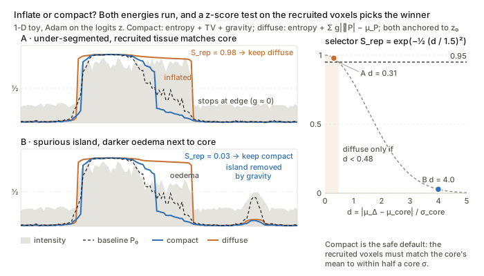
Figure. The orange diffuse mask stops where g\approx0 and the blue compact mask removes the island, and the right panel shows that S_{\text{rep}}>0.95 accepts the diffuse mask only when \lvert\mu_\Delta-\mu_{\text{core}}\rvert<0.48\,\sigma_{\text{core}}.
What to watch. Both energies are hand-assembled priors with fixed weights, not derived from a model of the shift. The selector compares only first and second intensity moments, and the paper does not say which channel. A recruited region with the same mean as the core but a different texture would pass the test.
W-PM-142 · CoRe-DA: Contrastive Regression for Unsupervised Domain Adaptation in Surgical Skill Assessment
Dimitrios Anastasiou, Razvan Caramalau, Jialang Xu et al. — arXiv:2603.29666
Core idea. The method adapts a skill-score regressor through pairwise score differences rather than absolute scores. A relative head predicts y_i-y_j for a pair of videos, and target scores are reconstructed by anchoring on a labelled source “exemplar”. The premise is that relative skill is more domain-invariant than the absolute scale. Adaptation to the unlabelled target comes from self-training that forces the absolute and relative pathways to agree, with a stop-gradient on the absolute branch.
Mathematical constructs.
- Two heads on a shared encoder. Each training sample is a triplet (x_S,x_E,x_T): source, exemplar and target. With encoder F and global average pooling (GAP) over K clips: \hat{y}^{\text{abs}}_i=R_{\text{abs}}(F(x_i)),\qquad \widehat{\Delta y}_{j-E}=R_{\text{rel}}\big(\mathrm{concat}[\mathrm{GAP}F(x_j);\mathrm{GAP}F(x_E)]\big), for i\in\{S,E,T\} and j\in\{S,T\}. The anchored reconstruction is \hat{y}^{\text{recon}}_j=\widehat{\Delta y}_{j-E}+\hat{y}^{\text{abs}}_E.
- Supervised losses (source only). \mathcal{L}^{\text{rel}}_{\text{sup}}=\frac1B\sum(\widehat{\Delta y}_{S-E}-(y_S-y_E))^2 and \mathcal{L}^{\text{abs}}_{\text{sup}}=\frac1B\sum(\hat{y}^{\text{abs}}_E-y_E)^2. The relative loss is the contrastive-regression term; the absolute loss fixes the score scale.
- Cross-head consistency on the source. \mathcal{L}^S_{\text{cons}}=\frac1B\sum(\hat{y}^{\text{recon}}_S-\hat{y}^{\text{abs}}_S)^2 stops the two heads from drifting apart.
- Target self-training. \mathcal{L}^T_{\text{cons}}=\frac1B\sum\big(\hat{y}^{\text{recon}}_T-\mathrm{sg}(\hat{y}^{\text{abs}}_T)\big)^2. The absolute head acts as a pseudo-labeller for the relative pathway, and the stop-gradient (SimSiam-style) is used to avoid collapse. The total loss is \alpha(\mathcal{L}^{\text{rel}}_{\text{sup}}+\mathcal{L}^{\text{abs}}_{\text{sup}})+\beta\mathcal{L}^S_{\text{cons}}+\gamma\mathcal{L}^T_{\text{cons}}.
- Test-time multi-exemplar estimator with background mixing. M exemplars are drawn stratified by score. Each exemplar’s background frame BG_m is its temporal median. The target is mixed as \tilde{x}_{T,m}=(1-\lambda)x_T+\lambda BG_m, a mixup-style interpolation towards source appearance. The target is scored with the true exemplar labels, \hat{y}^{\text{recon}}_{T,m}=\widehat{\Delta y}_{T-E,m}+y_{E,m}, and \bar{y}_T=\frac1M\sum_m\hat{y}^{\text{recon}}_{T,m}. The error therefore comes only from the relative head, averaged over anchors.
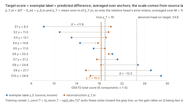
Figure. Each arrow is one vote \hat y_{T,m}=\widehat{\Delta y}_{T-E,m}+y_{E,m}, and their mean \bar y_T (orange line) lands near the truth while the shifted absolute head (grey) does not; the consistency loss pulls the other way during training.
What to watch. No divergence between domains is ever measured or minimised; domain invariance is argued, not enforced. The target loss has no label signal and can be satisfied by two heads that agree on wrong values. R_{\text{rel}} is not constrained to be antisymmetric or transitive, so it is not guaranteed to act as a true difference operator.
W-PM-180 · PROTON: Prototype-Based Test-Time Online OOD Detection for Medical VLMs
Abhijit Das, Nichula Wasalathilaka, Yifan Lu et al. — arXiv:2606.20913
Core idea. Softmax-based OOD scores such as MCM compress the embedding into one confidence scalar. Covariate-shifted images can be as confident as in-distribution images while lying elsewhere on the embedding hypersphere. PROTON builds class prototypes online from confidently self-labelled test embeddings and scores each sample by cosine distance to the nearest prototype. It then mixes this distance with MCM using a weight driven by the running variance of the MCM stream. Everything is training-free and gradient-free on a frozen VLM.
Mathematical constructs.
- MCM base score. Take \ell_2-normalised image embeddings e_t and cached class text embeddings \mathbf{T}\in\mathbb{R}^{C\times d}. Then p_t=\mathrm{softmax}(e_t^\top\mathbf{T}/\tau) and S_{\text{MCM}}(x_t)=-\max_c p_{t,c}, where higher means more OOD.
- Online prototype bank. Each class has a FIFO queue \mathcal{D}_c of size M. The embedding e_t is enqueued into \mathcal{D}_{\hat{c}}, \hat{c}=\arg\max_c p_{t,c}, only if \max_c p_{t,c}\ge\gamma, which is the confidence gate. The prototype is the renormalised mean direction: \mu_c=\frac{\bar{e}_c}{\lVert\bar{e}_c\rVert_2},\qquad \bar{e}_c=\frac{1}{\lvert\mathcal{D}_c\rvert}\sum_{e\in\mathcal{D}_c}e . This is the maximum-likelihood mean direction of a von Mises–Fisher model. The FIFO queue makes it a sliding-window estimate that tracks recent statistics.
- Prototype distance. S_{\text{proto}}(x_t)=1-\max_c e_t^\top\mu_c, the cosine distance to the nearest centroid. It is used only once every class holds K_{\min} samples; before that S=S_{\text{MCM}}.
- Variance-adaptive convex fusion. S_{\text{PROTON}}=\alpha_t S_{\text{MCM}}+(1-\alpha_t)S_{\text{proto}},\qquad \alpha_t=\alpha_{\max}-\sigma\big(100(\sigma_t^2-\sigma_0^2)\big)(\alpha_{\max}-\alpha_{\min}). \sigma_t^2 is the running variance of S_{\text{MCM}} and \sigma_0^2 is a reference value for an in-distribution-only stream. High variance, taken as a sign of confidently wrong covariate samples, moves weight to S_{\text{proto}}. The steep sigmoid acts as a smoothed switch.
- Welford’s recursion. The variance is computed exactly in one pass with O(1) memory. With \delta=S_t-\bar{S}: \bar{S}\leftarrow\bar{S}+\delta/n, M_2\leftarrow M_2+\delta(S_t-\bar{S}), \sigma_t^2=M_2/n.
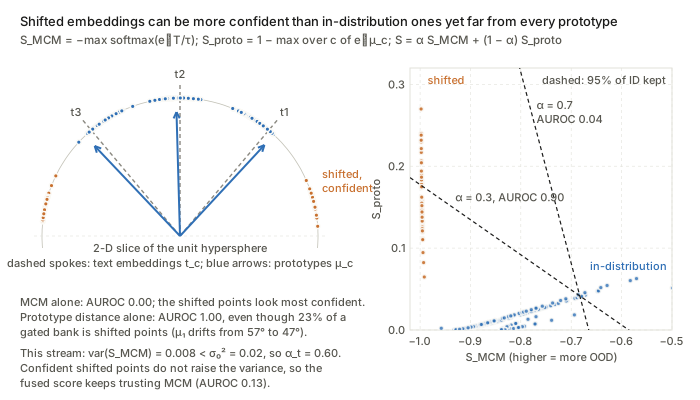
Figure. The orange points are the most confident under S_{\text{MCM}} but far from every prototype \mu_c, and the dashed boundaries show how \alpha_t trades the two scores off; confident shifted points shrink the MCM variance, so \alpha_t stays high.
What to watch. The bank is built by self-labelling, so confident OOD samples that pass the gate contaminate the prototypes, a form of confirmation bias. \sigma_t^2 is a cumulative variance over the whole stream, not a windowed one, so \alpha_t reacts slowly to late shifts. S_{\text{MCM}}\in[-1,-1/C] and S_{\text{proto}}\in[0,2] are on different scales, so the convex fusion is not calibrated. Each sample’s score also depends on the composition of the test stream.
W-PM-207 · JANUS: Anatomy-Conditioned Gating for Robust CT Triage Under Distribution Shift
Lavsen Dahal, Yubraj Bhandari, Geoffrey Rubin et al. — arXiv:2605.13813
Core idea. Attention pooling produces a convex combination of tokens, so it is invariant to token count. Size-defined findings such as organ volume or vessel calibre are therefore invisible in the pooled embedding; the authors call this the “geometric gap”. JANUS restores this information by computing segmentation-derived macro-radiomic scalars s_\ell per label. It uses them as a multiplicative sigmoid gate on the ROI-pooled visual embedding, a scale-only FiLM, so that measurements can attenuate visual evidence rather than merely add to it. The argument is that anatomy is protocol-invariant while appearance is not.
Mathematical constructs.
- Conditional model. The target is P(y\mid X,S) with partially observed labels y\in\{0,1,\varnothing\}^L and availability indicators \delta_\ell=\mathbb{1}[y_\ell\neq\varnothing].
- ROI-masked attention pooling. Token u_{t,i} is patch i of tri-slice t, and m_{t,i,\ell}\in\{0,1\} is the dilated ROI mask for label \ell. Then a_{t,i,\ell}=\frac{\phi_\ell(u_{t,i})+\beta_{\text{in},\ell}m_{t,i,\ell}}{\tau_\ell},\quad w_{t,i,\ell}=\underset{i:\,m_{t,i,\ell}=1}{\mathrm{softmax}}(a_{t,i,\ell}),\quad z_{v,\ell}=\frac1T\sum_{t=1}^T\sum_{i:\,m_{t,i,\ell}=1}w_{t,i,\ell}u_{t,i}. The weights are normalised per slice over ROI tokens and then averaged over slices.
- Anatomically guided gate. g_\ell=\sigma(W_{g,\ell}s_\ell+b_{g,\ell})\in[0,1]^d,\qquad z_{\text{gated},\ell}=z_{v,\ell}\odot g_\ell,\qquad \hat{y}_\ell=w_\ell^\top z_{\text{gated},\ell}+b_\ell . Here s_\ell is z-scored with training statistics. The logit \sum_k w_{\ell k}g_{\ell k}z_{\ell k} is a bilinear interaction between measurements and appearance. With b_g=2 at initialisation, \sigma(2)\approx0.88, so the gate starts almost open.
- Curriculum partial-label BCE. \mathcal{L}^{(e)}=\frac{\sum_\ell\big[\delta_\ell\,\mathrm{BCE}(p_\ell,y_\ell)+(1-\delta_\ell)w^{(e)}\mathrm{BCE}(p_\ell,0)\big]}{\sum_\ell\big[\delta_\ell+(1-\delta_\ell)w^{(e)}\big]} . The weight w^{(e)} ramps linearly from 0 to 0.3 between epochs 10 and 20, so missing labels are treated as increasingly weighted weak negatives.
- Physiological Veto Rate. With F_\ell=\{i: y_{i\ell}=0,\ p^{\text{ViT}}_{i\ell}\ge0.8\}, the set of confident baseline false positives, \mathrm{PVR}_\ell=\frac{1}{\lvert F_\ell\rvert}\sum_{i\in F_\ell}\mathbb{1}[p^{\text{JANUS}}_{i\ell}<0.5]. Selectivity is \mathrm{PVR}_\ell/\mathrm{TSR}_\ell, where \mathrm{TSR}_\ell=\Pr(p^{\text{JANUS}}_{i\ell}<0.5\mid y_{i\ell}=1).
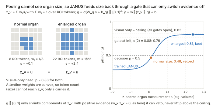
Figure. Both token grids pool to the same z_v, so only the measurement s separates the cases, and the gate g=\sigma(W_g s+b_g) vetoes the normal-sized case while staying under the visual-only ceiling: it can only switch evidence off.
What to watch. The in-ROI bias \beta_{\text{in},\ell}m is constant over the softmax support, so it cancels; the hard ROI restriction does all the work. Because g\in[0,1], the gate shrinks magnitudes rather than logits: it acts as a “veto” only when the attenuated components carry positive evidence (w_{\ell k}z_{\ell k}>0). The robustness argument also assumes the segmentation that produces s_\ell is itself invariant to the shift.