Weight Space Learning for Certifiable Few-shot Transfer Learning
Links
- arXiv:2502.06970 —
note this is the earlier version of the work, an ICLR
2025 workshop paper titled Model Diffusion for Certifiable Few-shot
Transfer Learning, same authors and same method. These notes
annotate the ICML 2026 camera-ready, which renames the method STEEL and
adds the LLM benchmarks.
make fetchwill pull the earlier version. - Inequalities and concentration — the finite-hypothesis bound used here is Hoeffding plus a union bound, covered there.
- Runnable
code — the bound arithmetic, including a rederivation of
Eq. 3 from Hoeffding.
make verifyruns it.
In one paragraph
You fine-tune CLIP on 16 examples per class and get 90% held-out accuracy. Can you guarantee a minimum accuracy on unseen data, of the sort a regulator might require? Today, no: every bound’s complexity term scales with the size of the searched hypothesis space, and for even a small continuous adapter that term swamps the [0,1] range of the loss. STEEL’s move is to stop optimising over a continuous space and select from a finite list: fit adapters to upstream tasks, train a diffusion model over them, then at test time sample |\Theta| candidates unconditionally and return whichever scores best on the support set. Complexity drops from d to \log|\Theta|, and the classical finite-hypothesis bound — elementary, and older than deep learning — becomes non-vacuous in the few-shot regime for the first time.
The spine of the argument
- Continuous hypothesis spaces make few-shot certificates vacuous, whatever the optimiser.
- Restrict the learner to return one of |\Theta| pre-committed candidates. Complexity becomes \sqrt{\log(|\Theta|/\epsilon)/2n}, and \log of a large number is small.
- Get the candidates from a diffusion model trained on upstream task adapters, so the class is rich enough to contain good solutions and can interpolate between upstream tasks.
- The bound is Hoeffding plus a union bound, so it holds uniformly over \Theta — which is precisely what licenses selecting the best candidate after seeing the support set.
- Everything else (hierarchical search, distribution shift, suboptimal selection) can only loosen the certificate, never invalidate it.
Setup and notation
| Symbol | Meaning |
|---|---|
| \Theta | the finite hypothesis set: adapters sampled from the diffusion model |
| \|\Theta\| | its size; 10k–20k in their experiments |
| d | number of continuous PEFT parameters (\approx 1000 for their LoRA-XS) |
| n | support set size (= 80 for 16-shot 5-way) |
| r(\theta), R(\theta) | empirical risk on the support set, and true risk |
| C | loss bound, 0 \le \ell \le C |
| \epsilon | certificate failure probability |
| n_d, T^* | difficult examples per class; the downstream task |
The arithmetic, which is the whole paper
Two certificates of the form R \le r + \text{complexity}:
\underbrace{C\sqrt{\frac{\log(|\Theta|/\epsilon)}{2n}}}_{\text{Eq. 3, finite class}} \qquad\text{vs}\qquad \underbrace{C\sqrt{\frac{d + 2\log d + \log(1/\epsilon)}{2n}}}_{\text{Eq. 7, continuous}}
Eq. 7 is the best case of the Lotfi et al. (2024) quantisation bound, assuming one bit per parameter, so it flatters the competition. At their 16-shot 5-way setting (n = 80):
| bound | complexity | verdict |
|---|---|---|
| continuous, d \approx 1000 | 2.52 | vacuous (loss is in [0,1]) |
| finite, \|\Theta\| = 20{,}000 | 0.284 | usable |
An 8.9× gap. These reproduce their Table 2 closely (reported min bounds 2.55 and 0.30), which also confirms d \approx 1000 for their adapters. The continuous bound does not drop below 1 until n \approx 508 — nowhere near few-shot.
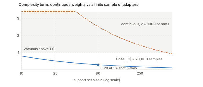
The logarithm also means the class size is almost free to grow:
code/bounds.py shows the complexity moving only from 0.218
to 0.324 as |\Theta| goes from 10^2 to 10^6.
The method
Upstream. Fit a PEFT adapter to each source task; treat \{\theta_i\} as samples from a distribution over “adapters that solve tasks from this family”; fit a diffusion model to it. That generator is the transferred meta-knowledge — the analogue of MAML’s initialisation \theta_0, but a distribution rather than a point.
Downstream. Given support set S^*: draw |\Theta| adapters unconditionally, score each on S^*, return \theta^* = \arg\min_{\theta\in\Theta} r(\theta). No gradients at test time. Learning is selection.
Two refinements. Search may be hierarchical (clustered, O(\log|\Theta|)) rather than exhaustive — a worse \theta^*, but the bound is unaffected. And a diffusion model rather than the raw model zoo, for compactness and because it can interpolate between upstream solutions; their ablations show it beats selecting from the zoo directly.
Why the bound is sound
“Use the support set to choose the model, then certify it on the same support set” sounds like cheating. It is not, for the classical reason.
Eq. 3 is Hoeffding plus a union bound. For one fixed \theta, Hoeffding gives \Pr(R - r > t) \le \exp(-2nt^2/C^2). Union over |\Theta| candidates and set the total failure probability to \epsilon:
t = C\sqrt{\frac{\log(|\Theta|/\epsilon)}{2n}} .
code/bounds.py rederives this numerically — plugging
t back gives |\Theta|e^{-2nt^2} = 0.0500 exactly. The
bound therefore holds simultaneously for every \theta \in \Theta, so you may pick whichever
you like after looking at the data. Paying \log|\Theta| is the price of that
freedom. The PAC-Bayes framing (uniform prior, Dirac posterior) is
optional dressing; this is the Occam bound.
The critical precondition is that \Theta is fixed before S^* is seen — and it is, because the samples are drawn unconditionally from a generator trained only on upstream tasks.
Two consequences the paper draws out well:
- The i.i.d.-task assumption affects tightness, not validity. The bound needs only S^* i.i.d. from the downstream task. Under distribution shift the sampled adapters fit poorly, r(\theta^*) rises, and the certificate is honestly bad — never wrong. Demonstrated with CUB→iNaturalist.
- You get a deployment decision. Gradient-based meta-learning hands you a model with no statement attached; here you read the certified risk and may decline to deploy.
Results
- Vision, 16-shot 5-way: 97–100% of episodes non-vacuous across four datasets. SGD and BBPT give 0%, every time. LoRA-Hub 35–100%, Meta-PB 0–97%.
- LLM (LaMP personalisation): 65% non-vacuous, vs 32% (LoRA-Hub) and 0% (SGD, MeZO).
- Scaling shots: at 64–128 shots on iNaturalist the certificate sits just 6% above empirical test error — genuinely tight, with far fewer examples than the ≥10k prior certification work needs.
The accuracy cost is real, and the paper undersells it. It describes STEEL as “within a small margin” of fine-tuning:
| Dataset | SGD | STEEL | gap |
|---|---|---|---|
| CUB | 90.3% | 88.4% | −1.9 |
| Aircraft | 65.6% | 61.4% | −4.2 |
| DTD | 88.0% | 81.5% | −6.5 |
| Flowers | 95.9% | 84.9% | −11.0 |
Eleven points is not a small margin. The honest framing: you are buying a certificate with accuracy, at a price between roughly 2 and 11 points.
What is genuinely clever
The inversion. The field’s usual move is here is an algorithm, find a tighter bound for it. This paper does the opposite: here is the tightest bound we have — elementary, and decades old — design an algorithm it applies to. The bound is not the contribution; making a competitive deep-learning method fit it is.
There is also an unusual consequence in their Figure 5: because complexity grows with |\Theta|, drawing more samples eventually hurts the certificate even while training error keeps falling. On DTD the best bound occurs after relatively few samples. “How hard should I search?” becomes an explicit, tunable trade-off that gradient descent simply does not have.
Questions and doubts
- \log|\Theta| is loose, and they know it. Many sampled adapters make near-identical predictions, so counting each as an independent hypothesis overpays. Their own suggested fix — a prediction-space covering number N(\Theta,\varepsilon) — would decouple certificate strength from raw sample count. That is the obvious next paper.
- Choosing |\Theta| looks unpaid-for. Figure 5 sweeps |\Theta| and observes where the bound is best, but that optimum depends on S^* through r(\theta). Selecting |\Theta| by reading the curve is model selection on the data, needing a further union bound over the grid. Cheap to fix (another log), but not addressed.
- Per-episode versus simultaneous. “% non-vacuous tasks” aggregates certificates each holding with probability 1-\epsilon individually. Fine as a per-deployment claim; not a guarantee across all episodes at once.
- Usefulness rests on an assumption the theory deliberately excludes. If no upstream task resembles the downstream one, the generator has nothing useful to sample. The bound stays valid and says so — correct behaviour, but it means practical value depends on coverage that the theory does not cover.
Takeaways
- Complexity entering as \log|\Theta| rather than d is the entire mechanism, and it is worth carrying as an intuition: searching a huge finite list is cheap; searching a small continuous space is not.
- The finite-hypothesis bound holds uniformly, which is exactly why data-dependent selection from a data-independent pool is legitimate. Everything hinges on \Theta being drawn before the support set is seen.
- Certification and accuracy are in tension here, with a measurable exchange rate. That is a more honest framing than “comparable performance”.
- Compare with the NTK notes: both escape “complexity scales with parameter count”, but by opposite routes — STEEL shrinks the class until the count is small, NTK shows the count was never the right measure.