Optimal transport and the Wasserstein distance
Links
- Interactive version: every section below has a widget you can play with there: sand being shovelled into holes, a draggable bakery→café map, the coupling heatmap with a Sinkhorn blur slider, W₁ vs. KL/JS, and point clouds flowing along optimal pairings.
- Wang et al. 2026, NTK-Selector: uses TSDS (Liu et al., 2024), an OT-based data-selection method, as a baseline. §8 below reads that definition symbol by symbol.
- Li et al. 2026, hyperbolic flow matching: flow matching, where OT pairings straighten the paths (§6).
- Gaussianity in practice: if embeddings are Gaussian, the W₂ distance between two of them has a closed form (§7).
- Peyré & Cuturi, Computational Optimal Transport (2019): readable and ML-oriented, with most of these pictures. Villani, Optimal Transport: Old and New (2009) is the deep-theory reference.
In one paragraph
Picture a probability distribution as a pile of sand, tall where there is a lot of probability. Optimal transport (OT) asks: what is the cheapest way to reshape pile \mu into pile \nu, if moving one grain a distance d costs d (or d^2)? The minimum cost is a distance between distributions, the Wasserstein distance. Unlike KL or Jensen–Shannon, it measures how far mass has to travel, not just whether the two densities disagree at a point. So it stays informative when the distributions don’t overlap at all, which is the usual situation for data on thin manifolds. That’s why it turns up in WGANs, FID, flow matching, domain adaptation and transferability estimation.
1. The idea: sand into holes
Pile \mu (the source) sits above ground. A set of holes shaped like \nu (the target) sits below. Both hold total mass 1. A way of shovelling assigns every grain to a hole. The optimal way minimises the average distance a grain travels, and that minimum is W_1(\mu,\nu), the earth mover’s distance.
In one dimension the optimal rule is: sort the grains left to right, sort the holes left to right, and match first with first, second with second, and so on. Paths never cross. Any matching where paths cross can be improved by swapping the two endpoints. A random matching criss-crosses and costs more.
2. A worked example with numbers
Three bakeries bake 30, 20 and 50 loaves. Three cafés need 40, 35 and 25. Shipping a loaf costs its distance C_{ij}. Divided by 100, that’s \mu=(0.3,0.2,0.5) and \nu=(0.4,0.35,0.25).
A transport plan is a table: “ship \gamma_{ij} loaves from bakery i to café j”. It has to obey two rules:
- row sums = supply: \sum_j\gamma_{ij}=\mu_i (each bakery ships out everything it baked);
- column sums = demand: \sum_i\gamma_{ij}=\nu_j (each café gets exactly what it needs).
OT picks, among all such tables, the one with the smallest \sum_{ij}C_{ij}\gamma_{ij}. A naive plan that fills café 1, then café 2, then café 3 (the north-west corner rule) obeys both rules but ignores distance, and costs more. Two things to notice in the interactive version:
- the optimal plan often splits one bakery’s output across two cafés;
- for m sources and n targets, an optimal vertex solution has at most m+n-1 non-zero cells, so plans are sparse.
3. Maps vs. plans (Monge vs. Kantorovich)
Monge (1781) asks for a map T: every grain at x goes to exactly one place T(x). The constraint is written T_\#\mu=\nu, “T pushes μ forward to ν”. In plain words: move every grain of \mu to T(\text{grain}), and the resulting pile must be exactly \nu. In deep learning terms, if X\sim\mu is an input and T is a network, then T_\#\mu is just the distribution of the outputs T(X). Formally, (T_\#\mu)(B)=\mu\big(T^{-1}(B)\big): the probability of landing in region B equals the probability of starting somewhere that T sends into B.
Maps have a problem. If \mu is one spike of mass 1 and \nu is two spikes of mass ½, no function can do it, because a function sends the whole spike to one point.
Kantorovich (1942) fixes this by allowing mass to split. Instead of a map, you choose a plan \gamma(x,y), which says how much mass goes from x to y. That’s the table from §2. The problem now always has a solution, and it is a linear program.
Brenier’s theorem says that when \mu has a density (no spikes) and the cost is \|x-y\|^2, the optimal plan doesn’t split anything after all: it is concentrated on the graph of a map y=T(x), and that map is the gradient of a convex function. So the two formulations agree in the nice case.
4. A plan is a joint distribution
Divide the plan by its total mass and \gamma is the joint distribution of a pair (X,Y) with
- marginal over y (row sums) equal to \mu, the distribution of X, and
- marginal over x (column sums) equal to \nu, the distribution of Y.
A joint distribution with prescribed marginals is a coupling. OT is choosing the coupling of \mu and \nu under which X and Y are closest on average:
\mathrm{OT}_c(\mu,\nu)=\min_{\gamma\in\Pi(\mu,\nu)}\ \mathbb E_{(X,Y)\sim\gamma}\big[c(X,Y)\big].
The interactive heatmap draws \gamma(x,y) with \mu up the side and \nu along the top. Its blur slider \varepsilon (entropic regularisation, below) interpolates between two extremes:
| \varepsilon | Plan | Meaning |
|---|---|---|
| 0 | a thin increasing curve | exact OT. A Monge map (Brenier), the sort-and-match rule of §1 |
| small | the curve with a soft halo | Sinkhorn. Slightly more expensive, but fast, GPU-friendly and differentiable |
| \to\infty | \mu(x)\,\nu(y) | the independent coupling. Still a valid plan (the marginals are right), but X and Y ignore each other |
5. Why ML likes Wasserstein distance
Let \mu=\mathrm{Unif}[-w/2,w/2] and let \nu be the same block shifted by \theta.
| Divergence | Value | What happens once \lvert\theta\rvert\ge w (no overlap) |
|---|---|---|
| W_1(\mu,\nu) | \lvert\theta\rvert | keeps shrinking as \nu moves closer, so the gradient points the right way |
| \mathrm{JS}(\mu,\nu) | \log 2\cdot\min(1,\lvert\theta\rvert/w) | stuck at \log 2, so the gradient is zero |
| \mathrm{KL}(\mu\Vert\nu) | \infty for every \theta\neq0 | infinite, no signal at all |
The JS value comes from a short computation. Where the blocks overlap, the two densities are equal and contribute nothing. On the non-overlapping fraction 1-o, with o=\max(0,1-|\theta|/w), each density is compared with the mixture m, where it is twice as large as m. That gives \mathrm{JS}=(1-o)\log 2.
This is the core argument of the Wasserstein GAN (Arjovsky, Chintala & Bottou, 2017). Real images and early generator samples live on thin, non-overlapping manifolds, so the flat-JS regime is the normal case, not a corner case.
6. Point clouds and straight-line flows
With samples instead of densities (n equally weighted points on each side), OT becomes an assignment problem: pair every source point with exactly one target point so that the mean squared distance is smallest. That minimum is W_2^2 between the two empirical distributions. (Birkhoff’s theorem is why the optimal plan is a permutation here rather than something split.)
Move each point along x_t=(1-t)\,x_0+t\,x_1. With the optimal pairing, paths are short and, for squared cost, two moving points never occupy the same place at the same time (W_2-optimal paths don’t collide). With random pairing, paths are long and tangled. Flow-matching models regress a velocity field along exactly these paths. Tangled paths mean a harder regression target and more integration steps at sampling time. That’s why OT-conditional flow matching (Tong et al., 2023) and multisample flow matching (Pooladian et al., 2023) pair noise with data by minibatch OT before training.
7. The formal definitions, piece by piece
Ingredients
| Symbol | Meaning | Picture |
|---|---|---|
| \mu on \mathcal X | source distribution | the sand pile, the bakeries, domain A |
| \nu on \mathcal Y | target distribution | the holes, the cafés, domain B |
| c(x,y) | cost of moving one unit of mass from x to y | distance on the map. Usually \lVert x-y\rVert or \lVert x-y\rVert^2 |
| \Pi(\mu,\nu) | couplings: joint distributions with marginals \mu,\nu | valid shipping tables |
Monge and Kantorovich
\text{Monge:}\quad \inf_{T:\,T_\#\mu=\nu}\ \int c\big(x,T(x)\big)\,d\mu(x), \qquad \text{Kantorovich:}\quad \min_{\gamma\in\Pi(\mu,\nu)}\ \int c(x,y)\,d\gamma(x,y).
\int c(x,T(x))\,d\mu(x) is just \mathbb E_{X\sim\mu}[c(X,T(X))], the average cost per grain. \gamma\in\Pi(\mu,\nu) means \gamma(A\times\mathcal Y)=\mu(A) and \gamma(\mathcal X\times B)=\nu(B), which are the row-sum and column-sum rules.
Discrete version (what code solves)
With weights a\in\mathbb R^n, b\in\mathbb R^m and cost matrix C_{ij}=c(x_i,y_j):
\min_{P\in\mathbb R_{\ge0}^{n\times m}}\ \sum_{i,j}C_{ij}P_{ij} \quad\text{s.t.}\quad P\mathbf 1_m=a,\quad P^\top\mathbf 1_n=b.
A linear program with nm unknowns. Exact solvers (network simplex) scale roughly cubically, which is why entropic regularisation matters in practice.
Wasserstein distance
W_p(\mu,\nu)=\Big(\min_{\gamma\in\Pi(\mu,\nu)}\ \mathbb E_{(X,Y)\sim\gamma}\lVert X-Y\rVert^p\Big)^{1/p}.
A genuine metric on distributions with finite p-th moment. W_1 is the earth mover’s distance, and W_2 is the one with the nice geometry (Brenier, displacement interpolation).
Closed forms worth memorising
- 1-D, with F^{-1},G^{-1} the quantile functions: W_p^p(\mu,\nu)=\int_0^1\big|F^{-1}(u)-G^{-1}(u)\big|^p\,du. This is “match quantile u with quantile u”, i.e. §1’s sort-and-match.
- Gaussians \mathcal N(m_1,\Sigma_1), \mathcal N(m_2,\Sigma_2): W_2^2=\lVert m_1-m_2\rVert^2+\operatorname{tr}\Big(\Sigma_1+\Sigma_2-2\big(\Sigma_2^{1/2}\Sigma_1\Sigma_2^{1/2}\big)^{1/2}\Big). This is exactly the FID score, computed on Inception features. It’s also the natural domain distance if you accept the Gaussian-embedding picture of Betser et al..
Entropic OT and Sinkhorn
\min_{P\in\Pi(a,b)}\ \sum_{ij}C_{ij}P_{ij}-\varepsilon H(P),\qquad H(P)=-\sum_{ij}P_{ij}\log P_{ij}.
The entropy rewards spread-out plans (the blur). The solution has the form P=\operatorname{diag}(u)\,K\operatorname{diag}(v) with K_{ij}=e^{-C_{ij}/\varepsilon}. Sinkhorn (Cuturi, 2013) finds u,v by alternately rescaling rows to match a and columns to match b. It uses only matrix–vector products, so it’s GPU-friendly and differentiable. For small \varepsilon, run it in the log domain to avoid underflow.
The next four subsections unpack this: where the form \operatorname{diag}(u)K\operatorname{diag}(v) comes from, what the alternating rescaling does, what \varepsilon changes, and the Sinkhorn divergence, which removes the bias that \varepsilon introduces.
Where the form \operatorname{diag}(u)\,K\operatorname{diag}(v) comes from
Without the entropy term, the best plan tends to use a few sharp routes, and with a distance cost it need not even be unique. Adding -\varepsilon H(P) makes the objective strictly convex, so there is exactly one best plan, and it is smooth in C, a and b.
To find it, give each row constraint a multiplier f_i and each column constraint a multiplier g_j, and set the derivative with respect to P_{ij} to zero:
C_{ij}+\varepsilon\log P_{ij}=f_i+g_j\quad\Longrightarrow\quad P_{ij}=e^{f_i/\varepsilon}\;e^{-C_{ij}/\varepsilon}\;e^{g_j/\varepsilon}=u_i\,K_{ij}\,v_j,
where u_i=e^{f_i/\varepsilon}, v_j=e^{g_j/\varepsilon} and K_{ij}=e^{-C_{ij}/\varepsilon}. In words: K is a table that is large for cheap routes and tiny for expensive ones, and the optimal plan is K with row i multiplied by a number u_i and column j multiplied by a number v_j. Instead of n\times m unknowns there are only n+m scaling factors.
Sinkhorn: rescale the rows, then the columns
The scaling factors are fixed by the two marginal conditions. Row sums must equal a and column sums must equal b:
u_i\,(Kv)_i=a_i,\qquad v_j\,(K^{\top}u)_j=b_j .
If v is held fixed, the first condition is solved at once by u=a/(Kv) (elementwise division). If u is held fixed, the second is solved by v=b/(K^{\top}u). Sinkhorn simply alternates:
u\leftarrow a\,/\,(Kv),\qquad v\leftarrow b\,/\,(K^{\top}u).
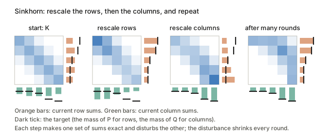
Each update makes one set of sums exactly right and spoils the other, but the spoiling shrinks every round. Geometrically, each update is the table closest to the current one (in the KL sense) that has the right row sums, then the right column sums: alternating projections between two constraint sets (Benamou et al., 2015). Each round costs two matrix–vector products, about nm operations, far less than solving the exact linear program. In practice it slows down as \varepsilon shrinks, and for small \varepsilon the entries of K underflow, which is why the log-domain version (below) is used.
What \varepsilon does
\varepsilon behaves like a temperature. Looking at the plan row of one source point, a small \varepsilon sends nearly all of its mass to the cheapest destination; a large \varepsilon spreads it over many.
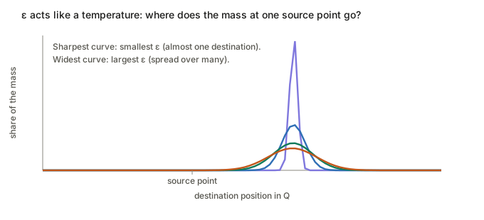
Across the whole plan this is the blur you see when \varepsilon is large, and the sharpening toward the exact optimal plan as it shrinks:
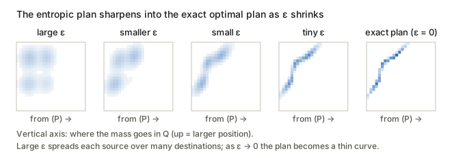
- Large \varepsilon: K is almost constant, so the plan approaches a\,b^{\top}, the “independent” plan that pays no attention to geometry.
- Small \varepsilon: the plan approaches the exact optimal plan. (For the squared cost in 1-D that plan is unique, which is why the right-hand panel is a clean curve.)
- The price: the entropic cost \langle P,C\rangle is always at or above the true optimal cost, so \varepsilon trades accuracy against speed and stability.
The Sinkhorn divergence: removing the bias
Write the regularised value as
\mathrm{OT}_\varepsilon(\mu,\nu)=\min_{P\in\Pi(a,b)}\ \langle P,C\rangle+\varepsilon\,\mathrm{KL}(P\,\|\,a\otimes b),
where a\otimes b is the independent plan with entries a_ib_j. (This differs from -\varepsilon H(P) only by a constant that depends on a and b, so the minimising plan is the same.) The problem: even \mathrm{OT}_\varepsilon(\mu,\mu) is not zero, because the entropy term makes the plan spread mass even when no moving is needed. So as a loss, it is not minimised by setting the generated distribution equal to the data.
The fix is to subtract each distribution’s value against itself (Feydy et al., 2019):
S_\varepsilon(\mu,\nu)=\mathrm{OT}_\varepsilon(\mu,\nu)-\tfrac12\,\mathrm{OT}_\varepsilon(\mu,\mu)-\tfrac12\,\mathrm{OT}_\varepsilon(\nu,\nu).
It is zero when \mu=\nu. For the squared-distance cost and any \varepsilon>0 it is also nonnegative and zero only then (Feydy et al., 2019), so it behaves like a proper distance.
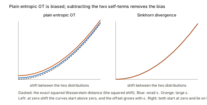
\varepsilon also sets what the divergence looks at. As \varepsilon\to0 it tends to the optimal-transport cost. As \varepsilon\to\infty, with the squared cost, it tends to the squared distance between the two means, since \mathbb E|X-Y|^2-\tfrac12\mathbb E|X-X'|^2-\tfrac12\mathbb E|Y-Y'|^2=\lVert\mathbb E X-\mathbb E Y\rVert^2 (here X,X' are independent draws from \mu and Y,Y' from \nu). In between it is a kernel distance (MMD) built from the cost. That is the sense in which the Sinkhorn divergence “interpolates between optimal transport and MMD”.
Using it as a training loss
Because every step is a plain tensor operation, the loss can be differentiated end to end, with no critic and no Lipschitz constraint (compare the WGAN critic above). The gradient has a simple reading: the derivative of \mathrm{OT}_\varepsilon with respect to a cost entry C_{ij} is the plan entry P_{ij}, so a generated point x_i is pulled toward the data points y_j it sends mass to,
\nabla_{x_i}\mathrm{OT}_\varepsilon=2\sum_j P_{ij}\,(x_i-y_j)\qquad\text{(squared cost)}.
An illustrative PyTorch version (log-domain updates; with the potentials f,g below, \mathrm{OT}_\varepsilon=\langle a,f\rangle+\langle b,g\rangle once the iteration has converged):
import numpy as np, torch

def ot_eps(x, y, eps=0.1, iters=50):
    n, m = len(x), len(y)
    C = torch.cdist(x, y) ** 2
    log_a = torch.full((n,), -np.log(n)); log_b = torch.full((m,), -np.log(m))
    f, g = torch.zeros(n), torch.zeros(m)
    for _ in range(iters):                       # alternate: rows, then columns
        f = -eps * torch.logsumexp(log_b[None, :] + (g[None, :] - C) / eps, dim=1)
        g = -eps * torch.logsumexp(log_a[:, None] + (f[:, None] - C) / eps, dim=0)
    return (log_a.exp() * f).sum() + (log_b.exp() * g).sum()

def sinkhorn_divergence(x, y, eps=0.1, iters=50):
    return ot_eps(x, y, eps, iters) - 0.5 * ot_eps(x, x, eps, iters) - 0.5 * ot_eps(y, y, eps, iters)

# training: generator G maps noise to points; the loss is differentiable through the iterations
#   loss = sinkhorn_divergence(G(torch.randn(256, 2)), real_batch)
#   opt.zero_grad(); loss.backward(); opt.step()
Since the real batch does not depend on the generator, the \mathrm{OT}_\varepsilon(y,y) term adds nothing to the gradient and can be dropped when only the gradient is needed. Two costs to keep in mind: each loss evaluation forms an n\times m cost table, and \varepsilon and the number of iterations have to be chosen together, since a small \varepsilon converges slowly.
Sources for this part
- Cuturi (2013), Sinkhorn Distances: Lightspeed Computation of Optimal Transport, NeurIPS: entropic regularisation for OT in machine learning.
- Peyré and Cuturi (2019), Computational Optimal Transport, Foundations and Trends in Machine Learning: the standard reference for everything above, including the log-domain form.
- Sinkhorn and Knopp (1967), Concerning nonnegative matrices and doubly stochastic matrices, Pacific Journal of Mathematics: the original alternating row and column scaling.
- Benamou, Carlier, Cuturi, Nenna and Peyré (2015), Iterative Bregman Projections for Regularized Transportation Problems, SIAM Journal on Scientific Computing: the alternating-projection view.
- Altschuler, Weed and Rigollet (2017), Near-linear time approximation algorithms for optimal transport via Sinkhorn iteration, NeurIPS: running-time guarantees.
- Genevay, Peyré and Cuturi (2018), Learning Generative Models with Sinkhorn Divergences, AISTATS: differentiating through Sinkhorn to train generators.
- Feydy, Séjourné, Vialard, Amari, Trouvé and Peyré (2019), Interpolating between Optimal Transport and MMD using Sinkhorn Divergences, AISTATS: the debiased divergence.
Duality: the shipping company’s view
\mathrm{OT}_c(\mu,\nu)=\max_{f,g}\Big\{\mathbb E_\mu[f(X)]+\mathbb E_\nu[g(Y)]\ :\ f(x)+g(y)\le c(x,y)\ \ \forall x,y\Big\}.
A shipping company charges f(x) to pick up at x and g(y) to drop off at y. To stay competitive, pickup plus dropoff can never exceed doing it yourself, c(x,y). The most it can earn equals your cheapest self-shipping cost. For W_1 the two potentials collapse into one 1-Lipschitz function (Kantorovich–Rubinstein):
W_1(\mu,\nu)=\sup_{\lVert f\rVert_{\mathrm{Lip}}\le1}\ \mathbb E_\mu[f(X)]-\mathbb E_\nu[f(Y)].
That f is the WGAN critic, kept 1-Lipschitz by weight clipping or a gradient penalty.
8. Reading a paper’s OT definition (data-selection example)
Data-selection papers state the discrete problem in their own notation. This version (it reads like TSDS, Liu et al., 2024, the OT baseline in NTK-Selector) is §7’s discrete problem with different letters:
\begin{aligned}&\min_{\gamma\in\mathbb R_{\ge0}^{|U|\times|V|}}\ \sum_{i=1}^{|U|}\sum_{j=1}^{|V|}\gamma_{ij}\,f(u_i,v_j)\\ &\text{s.t.}\ \ \sum_{j=1}^{|V|}\gamma_{ij}=\mu_i\ \ \forall i,\qquad \sum_{i=1}^{|U|}\gamma_{ij}=\nu_j\ \ \forall j.\end{aligned}
| Paper symbol | Plain meaning | In the bakery example (§2) |
|---|---|---|
| (A,f), a metric space | a finite set of examples A with a distance f between any two, e.g. between embeddings | the map, f = straight-line distance |
| U\subseteq A, points u_i | source examples (e.g. a candidate pool) | bakeries |
| V\subseteq A, points v_j | target examples (e.g. a small target-task set) | cafés |
| \mu_i=\mu(u_i) | mass on u_i. Uniform would be 1/\lvert U\rvert | supply ÷ 100 |
| \nu_j=\nu(v_j) | mass on v_j | demand ÷ 100 |
| \gamma\in\mathbb R_{\ge0}^{\lvert U\rvert\times\lvert V\rvert} | table, \gamma_{ij} = mass moved from u_i to v_j | the plan |
| \sum_{ij}\gamma_{ij}f(u_i,v_j) | total cost, mass × distance | total cost |
| \sum_j\gamma_{ij}=\mu_i | everything at u_i is shipped out | row sums |
| \sum_i\gamma_{ij}=\nu_j | every v_j gets exactly its share | column sums |
Two remarks help when reading these papers:
- U and V living in one space A just means a single f compares any source example with any target example. In practice f is a distance in some pretrained embedding space, and the OT answer is only as meaningful as that space.
- Why OT and not nearest neighbours. With f a metric, the optimal value is W_1(\mu,\nu). If a method gets to choose the weights \mu on the pool (e.g. mass only on selected examples), making W_1 small means picking candidates whose distribution covers the target’s. The column constraints force every target example to be served, so selections cannot all pile up near one popular target region. That’s a different objective from grabbing each target point’s nearest neighbours. (I haven’t checked how TSDS itself parametrises and optimises this; that’s for its own annotation.)
9. Where it shows up
- Generative models: WGAN trains against W_1 via the dual. FID is W_2 between Gaussian fits.
- Flow matching: minibatch-OT couplings straighten paths (Tong et al., 2023; Pooladian et al., 2023). Related: Li et al. 2026.
- Domain adaptation: Courty et al. (2017) align source and target features with an OT plan.
- Transferability / dataset distance: OTDD (Alvarez-Melis & Fusi, 2020) and OTCE (Tan et al., 2021) are OT-based cousins of LEEP, LogME and H-score.
- Libraries:
POT(Python Optimal Transport),geomloss,ott-jax.
Cheat sheet
| Term | One line |
|---|---|
| Optimal transport | cheapest rearrangement of \mu into \nu under a per-unit cost c(x,y) |
| Plan / coupling \gamma | joint distribution of (X,Y) with marginals \mu,\nu. In code, a matrix with fixed row and column sums |
| Map T | each x goes to one T(x). Can’t split mass. Exists in the nice case (Brenier) |
| Pushforward T_\#\mu | the distribution of T(X) when X\sim\mu |
| W_p | \big(\min_\gamma\mathbb E\lVert X-Y\rVert^p\big)^{1/p}. Measures travel distance, stays informative without overlap |
| Earth mover’s distance | another name for W_1 |
| Entropic OT / Sinkhorn | OT with a blur -\varepsilon H(P). Fast and differentiable. \varepsilon\to0: exact, \varepsilon\to\infty: \mu\otimes\nu |
| Dual potentials f,g | pickup and dropoff prices with f+g\le c. For W_1, a single 1-Lipschitz critic |