Neural Tangent Kernel: Convergence and Generalization in Neural Networks
Links
- arXiv:1806.07572 — preprint (the PDF in circulation is usually the 2020 revision of the NeurIPS 2018 paper).
- Inequalities and concentration — the background page; the CLT and concentration tools used here live there.
- Runnable
code — the NTK in numpy, with both theorems checked
numerically.
make verifyruns it. - Fort et al. 2020 — measures how far real training departs from this limit, and when. The short answer: the first two to three epochs.
- Column, null & residual spaces — the “\Delta^0_f never moves” statement in two dimensions: gradient descent cannot change the null-space part of its iterate.
In one paragraph
Training a network minimises C(F(\theta)), which is badly non-convex in \theta. But C is convex as a functional of the function f_\theta — all the non-convexity lives in the parametrisation, not the objective. So watch f_\theta instead. By the chain rule, gradient descent on parameters is gradient descent in function space with respect to the kernel \Theta(x,x') = \langle\nabla_\theta f_\theta(x), \nabla_\theta f_\theta(x')\rangle. That identity is exact at any width. The paper’s contribution is that in the infinite-width limit this kernel becomes deterministic (Theorem 1) and stops moving during training (Theorem 2), which turns training into a linear ODE in function space with a known, fixed kernel — and makes a wide network, trained to convergence on least squares, exactly kernel regression.
The spine of the argument
- Reframe: track f_\theta, not \theta. The cost is convex there.
- The chain rule gives \partial_t f_{\theta(t)} = -\nabla_{\Theta}C, a kernel gradient. The kernel is what extends the functional derivative — defined only on the data — to every other input, so it is exactly what governs behaviour off the training set.
- Warm-up (§3.1): for a linear random-feature model, this is exact and the tangent kernel converges to a fixed K by the law of large numbers. A wide network is this, except the features depend on \theta.
- Theorem 1: at initialisation the NTK converges in probability to a deterministic \Theta^{(L)}_\infty given by an explicit recursion.
- Theorem 2: it stays there during training, uniformly on [0,T].
- Consequence (§5): for least squares the function-space dynamics are linear, diagonal in the kernel principal components, and converge to the kernel ridge / GP posterior mean.
Setup and notation
| Symbol | Meaning |
|---|---|
| F^{(L)} : \mathbb{R}^P \to \mathcal{F} | realisation map, parameters \to function |
| f_\theta = \tilde\alpha^{(L)} | the network function; the output is a preactivation |
| n_0,\dots,n_L, P | layer widths and total parameter count |
| \beta | bias scaling, tuning bias influence against weights (\beta=0.1 in their experiments) |
| p_{in} | input distribution; here the empirical measure on a finite dataset |
| \langle f,g\rangle_{p_{in}} | \mathbb{E}_{x\sim p_{in}}[f(x)^\top g(x)] |
| \Sigma^{(L)} | NNGP kernel — covariance of the function at initialisation |
| \Theta^{(L)} | NTK — governs the training dynamics; a different object |
| \dot\Sigma^{(L+1)} | \mathbb{E}[\dot\sigma(f(x))\dot\sigma(f(x'))], the derivative kernel |
| \Pi | f \mapsto \Phi_K(\langle f,\cdot\rangle_{p_{in}}), whose eigenfunctions are the kernel PCs |
| \lambda_i | eigenvalue of \Pi; at most N n_L are positive |
The parametrisation is not cosmetic
They use
\tilde\alpha^{(\ell+1)} = \tfrac{1}{\sqrt{n_\ell}}W^{(\ell)}\alpha^{(\ell)} + \beta b^{(\ell)}, \qquad W, b \sim \mathcal{N}(0,1),
rather than LeCun initialisation. Their Remark 1 is explicit that the representable functions are the same, but the derivatives \partial_{W}F^{(L)} are scaled by 1/\sqrt{n_\ell}. Since the NTK is built from those derivatives, this scaling is what makes the limit exist at all. Different scalings (mean-field, μP) give different infinite-width limits — ones in which features do move. The NTK regime is one corner of a family, not “the” infinite-width theory.
Kernel gradient: the mechanism
A kernel K induces a map \Phi_K from the dual \mathcal{F}^* to \mathcal{F}, and
\nabla_K C\big|_{f_0}(x) = \frac{1}{N}\sum_{j} K(x,x_j)\, d\big|_{f_0}(x_j).
The functional derivative \partial^{in}_f C only knows the training points; the kernel is what carries it to arbitrary x. Along kernel gradient descent,
\partial_t C\big|_{f(t)} = -\big\lVert d|_{f(t)}\big\rVert_K^2,
so convergence to a critical point is guaranteed whenever K is positive definite with respect to \lVert\cdot\rVert_{p_{in}}. Convergence has become a positive-definiteness question, which is why Proposition 2 matters.
Theorem 1 — the kernel becomes deterministic
\Theta^{(1)}_\infty = \Sigma^{(1)}, \qquad \Theta^{(L+1)}_\infty = \Theta^{(L)}_\infty\,\dot\Sigma^{(L+1)} + \Sigma^{(L+1)},
with \Sigma^{(1)}(x,x') = \tfrac{1}{n_0}x^\top x' + \beta^2 and \Sigma^{(L+1)} = \mathbb{E}_{f\sim\mathcal{N}(0,\Sigma^{(L)})}[\sigma(f(x))\sigma(f(x'))] + \beta^2.
Random at any finite width; deterministic in the limit, depending only on \sigma, depth and initialisation variance — not on the draw.
Their Remark 4 gives the recursion its meaning: \Sigma^{(L+1)} is the learning contributed by the last layer’s weights, while \Theta^{(L)}_\infty\dot\Sigma^{(L+1)} is the backpropagated contribution of all lower layers. This is not a “only the last layer trains” result.
Theorem 2 — and why it is surprising
The NTK stays at \Theta^{(L)}_\infty uniformly on [0,T], provided \int_0^T \lVert d_t\rVert\,dt is stochastically bounded (which least squares satisfies, since \lVert f^*-f\rVert decreases).
Weights move. The function changes — it learns. Yet the kernel does not budge. Remark 4 again supplies the resolution: each individual activation’s variation shrinks with width, but their collective variation stays O(1).
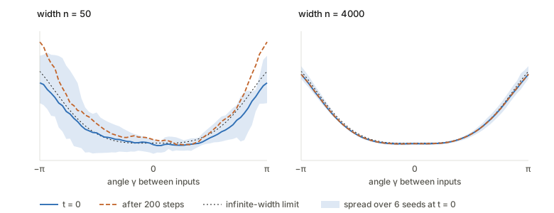
Checked numerically
code/ntk.py implements the forward and backward passes
for their exact parametrisation and assembles \Theta from the backprop deltas, alongside
the closed-form arccos kernels for \Sigma and \dot\Sigma. Depth 4, inputs on the unit
circle, as in their Figure 1:
| width | rel. error vs the Theorem 1 recursion | NTK drift over 200 GD steps | final loss |
|---|---|---|---|
| 50 | 0.229 | 38.3% | 0.00102 |
| 200 | 0.129 | 12.3% | 0.00057 |
| 1000 | 0.075 | 2.7% | 0.00051 |
| 4000/5000 | 0.039 | 0.8% | 0.00042 |
Initialisation error decays like 1/\sqrt n; drift decays faster, roughly like 1/n. And the loss falls to essentially the same value at every width — so the wide network learns just as well while its kernel stays frozen to within one percent. That juxtaposition is the content of Theorem 2 made concrete.
Section 5 — where the reframe pays off
For least squares the function-space ODE is linear:
f_t = f^* + e^{-t\Pi}(f_0 - f^*), \qquad f_t = f^* + \Delta^0_f + \sum_i e^{-t\lambda_i}\Delta^i_f .
The eigenfunctions of \Pi are the kernel principal components of the data, and each error component decays at its own rate \lambda_i. Three readings:
- Early stopping is spectral filtering. Stopping at time t fits the directions with \lambda_i \gg 1/t and leaves the rest. Since low-\lambda directions are the high-frequency, noisier ones, this is a principled account of a practitioner’s heuristic.
- \Delta^0_f never moves: it lies in the null space of \Pi: directions the kernel cannot see are never learned, at any t.
- At t\to\infty, f_\infty(x) = \kappa_x^\top \tilde K^{-1}y^* + (f_0(x) - \kappa_x^\top \tilde K^{-1}y_0). The first term is the GP posterior mean under prior \mathcal{N}(0,\Theta_\infty), equivalently kernel ridge regression as \lambda\to 0; the second is a zero-mean fluctuation vanishing on the training points. Ensemble a few networks and the fluctuation cancels: you get kernel regression exactly.
Proposition 2 closes the convergence argument: for non-polynomial Lipschitz \sigma and data on the sphere, \Theta_\infty is positive definite for L \ge 2. Non-polynomiality is load-bearing — the appendix notes that for polynomial \sigma, \Theta^{(2)} is not positive definite.
The catch, and the literature it spawned
A constant NTK means the feature map is constant, so the infinitely wide network does not learn features. It is a fixed random-feature model, and all “learning” is choosing coefficients in a basis fixed at initialisation.
That is a precise statement about what this limit does not model. Representation learning lives entirely in the kernel’s movement, which this limit sends to zero. The numbers above make it concrete: the width-50 network moved its kernel by 38% while matching the width-4000 network’s loss. Real networks are much closer to the former, and NTK regression empirically underperforms trained networks on hard tasks — usually read as evidence that feature learning does real work this limit discards.
Questions and doubts
- T is finite. Constancy is uniform on [0,T] given a bounded \int\lVert d_t\rVert dt. It is not a statement at fixed width as t\to\infty, and the order of the two limits matters more than the paper dwells on.
- No rates. Theorems 1 and 2 give convergence without
explicit n-dependence, so “how wide is
wide enough” is unanswered. The 1/\sqrt
n and \approx 1/n above are
measurements from
code/ntk.py, not their theorems. - p_{in} is the empirical measure on a finite dataset throughout, so the “function space” is effectively \mathbb{R}^N — a less grand object than the framing suggests.
- Fully connected only. Convolutional and attention NTKs came later, with different recursions.
- The parametrisation is a modelling choice presented almost in passing (Remark 1), yet it selects which infinite-width limit you get. A reader could finish the paper without realising the feature-learning regimes were excluded by a 1/\sqrt{n_\ell}.
Takeaways
- Gradient descent on parameters is exactly kernel gradient descent in function space. That identity is free; the theorems are about the kernel becoming knowable.
- Wide networks train to global minima not because the loss landscape is benign but because, in the right coordinates, the problem is convex and the dynamics linear.
- The kernel determines behaviour off the training set, so generalisation questions become questions about a kernel’s spectrum — and complexity stops scaling with parameter count.
- Early stopping, kernel PCA and the GP posterior all fall out of one linear ODE.
- The limit’s central weakness is its central assumption: a frozen kernel is a frozen feature map. Everything interesting about representation learning is in the residual this theory discards.