Difficult Examples Hurt Unsupervised Contrastive Learning
Links
- OpenReview forum — the ICLR 2026 venue page, with the reviews and discussion.
- arXiv:2501.01317 —
preprint.
make fetchpulls the PDF from here. - HaoChen et
al. 2021 — the notes on the paper this one builds on; the
spectral contrastive loss, the augmentation graph and the
4δ/(1−λ) + 8δbound all come from there. - Wang & Isola 2020 — where the alignment / uniformity decomposition of the contrastive loss comes from.
- Inequalities and concentration — background page collecting the tools these proofs run on (Cheeger, Donsker–Varadhan, Rademacher, Davis–Kahan and the rest).
Yi-Ge Zhang, Jingyi Cui, Qiran Li and Yisen Wang, Difficult Examples Hurt Unsupervised Contrastive Learning: A Theoretical Perspective, ICLR 2026. Full subtitle omitted from the title field for brevity.
In one paragraph
In supervised learning, the examples near the decision boundary are the valuable ones. In unsupervised contrastive learning they are not merely useless — deleting them improves downstream accuracy, even though it shrinks the training set. This paper explains why. It models the augmentation graph with just three similarity levels (\alpha within class, \beta across classes, \gamma across classes when both endpoints sit near the boundary), computes the spectrum of the resulting adjacency matrix in closed form, and reads off linear-probing error bounds. Difficult examples show up as a \gamma > \beta gap that raises the relevant eigenvalue and therefore the error bound. The same framework then explains three fixes — deleting the examples, adding a margin to difficult pairs, and scaling their temperature — each of which edits the similarity matrix in a different algebraic way.
The spine of the argument
- Analyse the spectral contrastive loss rather than InfoNCE, because it is exactly a matrix factorisation objective: minimising it computes the best rank-k approximation of the normalised augmentation-graph adjacency matrix \bar A.
- Linear-probing error is therefore controlled by the spectrum of \bar A, specifically by \lambda_{k+1}: error \le 4\delta/(1-\lambda_{k+1}) + 8\delta (HaoChen et al.).
- Model \bar A with three similarity levels, so its eigenvalues come out in closed form via Kronecker products.
- Difficult examples raise \lambda_{k+1}, hence a strictly worse bound (Thm 3.3 vs 3.4). The damage is governed by \gamma - \beta.
- Each remedy is a different edit to the target matrix: removal shrinks it (n \to n-n_d), margin tuning subtracts \bar M, temperature scaling multiplies elementwise by T. Choose the edit so the difficult entries land back on \beta and the damage is undone.
Everything hinges on step 1. Without the exact matrix-factorisation equivalence there is no spectrum to compute and no bound to read off.
Setup and notation
| Symbol | Meaning |
|---|---|
| \bar x \in \bar{\mathcal{X}} = \mathbb{R}^d | a natural (un-augmented) data point |
| A(\cdot \mid \bar x) | augmentation distribution given \bar x |
| \mathcal{X} | set of all augmented data; finite but exponentially large |
| n | number of augmented samples per class |
| r+1 | number of classes, so \lvert\mathcal{X}\rvert = n(r+1) |
| n_d, \mathcal{D}_d | difficult examples per class, and the set of them; n_e := n - n_d |
| k | feature dimension of the encoder f |
| \delta | labelling error in Assumption 3.1 (labels recoverable from augmentations) |
| w_{x,x'} | edge weight \mathbb{E}_{\bar x}[A(x\mid\bar x)A(x'\mid\bar x)]; \sum_{x,x'} w_{x,x'} = 1 |
| w_x | degree, \sum_{x'} w_{x,x'} |
| A, D, \bar A | adjacency (w_{x,x'}), degree \operatorname{diag}(w_x), normalised D^{-1/2} A D^{-1/2} |
| \lambda_{k+1} | the (k{+}1)-th largest eigenvalue of \bar A — every bound in the paper is a function of this one number |
| \alpha | similarity between two distinct same-class samples |
| \beta | similarity between two different-class samples, neither of them difficult |
| \gamma | similarity between a matched pair of different-class difficult samples |
| c_2 | (1-\alpha) + n\alpha + nr\beta — the degree w_x of an easy node |
| c_1 | c_2 + r(\gamma-\beta) — the degree w_x of a difficult node |
| c_0 | (1-\alpha) + n\alpha + (n-n_d)r\beta (as stated in Thm 4.3; see Questions below) |
| m_{x,x'}, M, \bar M | margin per pair, the margin matrix, and \bar M = D^{1/2} M D^{1/2} |
| \tau_{x,x'}, T | temperature per pair, and the temperature matrix |
| \sigma, \rho | the empirical margin and temperature-scaling factors in Eqs. 14–15 |
| p_{i,j} | indicator that the pair (x_i, x_j) was flagged difficult |
| \omega | mixing ratio in the \omega-Mixed CIFAR-10 experiments |
| \epsilon, \varepsilon_{ij}, W | noise scale, i.i.d. symmetric mean-0 variance-1 noise, and the resulting Wigner matrix |
The three similarity levels, and why \beta < \gamma < \alpha < 1
Self-similarity is 1 by definition, which anchors the scale. Same-class pairs should be the most similar of the rest, giving \alpha. Different-class pairs are less similar, and they split in two: if at least one endpoint sits near the class boundary the pair is difficult and gets the larger value \gamma; otherwise it is easy and gets \beta. Hence the ordering. The entire effect studied in the paper lives in the single gap
\gamma - \beta \;>\; 0,
and setting \gamma = \beta collapses every “with difficult examples” result back to its “without” counterpart. That is the cleanest way to read the theory: \gamma - \beta is the dial labelled “how much do difficult examples hurt”.
One structural detail that is easy to miss and matters for the constants: the difficult pairs are matched by index. Sample l of class i is \gamma-similar to sample l of class j, and to nothing else outside its class. So a difficult node has exactly r \gamma-neighbours — one per other class — and r(n-1) \beta-neighbours. That is where c_1 = c_2 + r(\gamma-\beta) comes from, with the coefficient r and not r n_d.
How \alpha, \beta, \gamma are measured, and the Table 10 trends
These are population constants in the theory, but the appendix estimates them empirically: train the model, then average cosine similarities over each group of pairs — same-class pairs for \alpha, different-class pairs with no flagged difficult endpoint for \beta, and different-class pairs containing a flagged difficult endpoint for \gamma. Difficult examples are flagged as the 8% of each class with the smallest gap between the top two softmax outputs.
On \omega-Mixed CIFAR-10, as the mixing ratio rises:
| Mixing ratio | 0% | 10% | 20% | 30% |
|---|---|---|---|---|
| accuracy (%) | 88.3 | 88.0 | 87.7 | 86.2 |
| \alpha | 47.2 | 44.0 | 41.2 | 38.7 |
| \beta | 19.1 | 19.5 | 20.1 | 20.8 |
| \gamma | 20.9 | 22.1 | 23.1 | 24.1 |
| \gamma - \beta | 1.80 | 2.60 | 3.00 | 3.30 |
| eigenvalue (\times 10^{-5}) | 2.93 | 3.36 | 3.58 | 3.72 |
\alpha falls because a pixel-mixed image nominally belongs to one class while carrying content from another, so it is a poor match for its own class-mates. Each class becomes internally more heterogeneous, and the average within-class similarity drops.
\beta and \gamma both rise because mixing degrades the representation globally: the encoder trained on contaminated data separates classes less well, so all cross-class pairs look more alike. Two further effects push the same way — the 8% selector is a fixed budget and cannot capture every mixed image, so some leak into the “easy” pool and lift \beta; and genuinely boundary-straddling images are exactly what raises \gamma.
\gamma rises faster than \beta, which is the point: \gamma-\beta nearly doubles from 1.80 to 3.30. Theorem 3.4 predicts a worse bound as that gap widens, and the measured \lambda_{k+1} duly climbs while accuracy falls. The table is the empirical validation of Theorem 3.4.
Worth noting that the paper emphasises \gamma - \beta but \alpha’s decline is doing independent work. Since
\lambda_{k+1} = \frac{1-\alpha}{(1-\alpha) + n\alpha + nr\beta},
a falling \alpha raises the numerator and lowers the denominator (its derivative in \alpha is n-1 > 0), so it pushes \lambda_{k+1} up on its own. The useful signal \alpha - \beta collapses from 28.1 to 17.9 across the table — faster in relative terms than \gamma-\beta grows. Mixing does not simply add confusable pairs; it compresses the whole similarity distribution.
Spectral contrastive loss vs InfoNCE
The loss analysed throughout is HaoChen et al.’s spectral contrastive loss,
\mathcal{L}_{\mathrm{Spec}}(f) := -2\,\mathbb{E}_{x,x^+}\big[f(x)^\top f(x^+)\big] + \mathbb{E}_{x,x'}\Big[\big(f(x)^\top f(x')\big)^2\Big].
Both this and InfoNCE are “attract positives, repel everything else”, and the attraction terms are the same linear inner product. All the differences are in the repulsion:
| InfoNCE | Spectral contrastive | |
|---|---|---|
| repulsion | \log\sum_j \exp(\langle u, v_j\rangle/\tau) | \big(f(x)^\top f(x')\big)^2 |
| coupling between negatives | multiplicative, all-pairs through the partition function | none; a plain expectation over independent x, x' |
| embedding constraint | \ell_2-normalised, so inner products are cosines on S^{d-1} | unnormalised; the norm carries \sqrt{w_x} and is meaningful |
| temperature | \tau is intrinsic | absent from the base form (reintroduced per-pair in Sec. 4.3) |
| batch dependence | denominator sums over the batch, giving an O(N^{-1/2}) finite-batch bias | already a population quantity |
| closed form for the minimiser | none; characterised only through kernel or limit arguments | exact: see below |
The last row is the reason for the substitution. With F = \big(\sqrt{w_x}\, f(x)\big)_{x \in \mathcal{X}},
\mathcal{L}_{\mathrm{mf}}(F) := \big\lVert \bar A - F F^\top \big\rVert_F^2 = \mathcal{L}_{\mathrm{Spec}}(f) + \text{const}.
Minimising the loss is literally computing the best rank-k approximation of \bar A, so the minimiser’s columns span the top-k eigenvectors of \bar A and contrastive learning becomes spectral clustering of the augmentation graph. That is what makes the rest of the paper possible: once you can write \bar A’s eigenvalues in closed form, you get a bound. InfoNCE admits no such identity. The substitution is licensed by Balestriero & LeCun (2022), Johnson et al. (2022) and Tan et al. (2024), which show the two losses share the same population minimum up to kernel reparametrisation.
A useful contrast with Betser et al. (2026), analysed elsewhere in this repo: that paper attacks population InfoNCE head-on and gets -\alpha\,\mathbb{E}[u \cdot v] + \Phi(\mu) with \Phi a log-sum-exp energy on the sphere. Same two-term structure; the log-sum-exp repulsion buys a statement about the distribution of representations, while the quadratic repulsion buys a statement about the spectrum of a graph. Neither is strictly stronger.
Why add random terms to the similarity values (Section 3.2)
The idealised A has exactly three distinct off-diagonal values. That is a rigidly block-symmetric matrix, and no real similarity matrix looks like it: real matrices have a distinct value in every entry and a spread-out spectral bulk rather than a handful of spikes. The relaxation replaces a_{ij} with
\tilde a_{ij} = a_{ij} + \epsilon \cdot \varepsilon_{ij}, \qquad \varepsilon_{ij} = \varepsilon_{ji} \ \text{i.i.d., mean } 0, \ \text{variance } 1,
keeping \tilde a_{ii} = 1. Five things this buys:
- It tests whether the conclusion is an artefact of exact symmetry. A result that held only for a perfectly rigid matrix would be suspect. The generalised Theorems B.4/B.5 show it survives.
- The noise is a Wigner matrix, so the perturbation is analysable. Symmetric, i.i.d., mean zero, unit variance is precisely the definition. Its spectrum obeys the semicircle law, so A + \epsilon W has the original spikes plus a controlled bulk — which is why the generalised bounds pick up an explicit \epsilon term with x_0 solving a Kepler equation, rather than becoming intractable.
- Mean zero leaves the degrees alone. Since \mathbb{E}\varepsilon_{ij} = 0, the degree matrix \tilde D \to D as n(r+1) \to \infty, so normalisation is asymptotically unaffected and the authors can apply the perturbation directly to \bar A for convenience.
- It reinterprets \alpha, \beta, \gamma as means rather than exact values. This matters because that is exactly how they are estimated in Table 10 — group averages. The relaxation is what reconciles the theory’s three constants with the measurement procedure.
- It shows what must stay small. The whole argument rests on a gap between \lambda_{r+1} and \lambda_{r+2}; the generalised bound degrades as \epsilon grows, with an extra -\frac{x_0 \epsilon}{(1-\alpha)+n(\alpha+r\beta)} in the denominator. So the model is honest about needing the idealisation to be a small perturbation.
Note the -\epsilon \cdot \operatorname{diag}(\varepsilon_{ii}) term in Eq. 62: a Wigner matrix carries diagonal noise too, and self-similarity must stay exactly 1, so it is subtracted back off.
Deconstructing Theorem 4.3
What it claims. There is a specific choice of margins under which margin-tuned contrastive learning on data containing difficult examples achieves exactly the error bound of plain contrastive learning on clean data: \mathcal{E}_M = \mathcal{E}_{w.o.}. An equality, not an improvement — the damage is fully undone.
It is easiest to read backwards, in five layers.
Layer 1 — what the two quantities are. Both are the RHS of a linear-probing bound of the form 4\delta/(1-\lambda_{k+1}) + 8\delta. So proving them equal means proving the two training problems have the same \lambda_{k+1}.
Layer 2 — what a margin actually does (Theorem 4.2). Adding m_{x,x'} inside the squared repulsion term gives
\mathcal{L}_{\mathrm{mf}-M}(F) = \big\lVert (\bar A - \bar M) - F F^\top \big\rVert_F^2 .
At the population level margins do exactly one thing: replace the factorisation target \bar A with \bar A - \bar M. Nothing else about the problem changes, and everything downstream depends on the target only through its spectrum.
Layer 3 — the design goal. So choose \bar M to make
\bar A - \bar M = \bar A_{w.o.},
the normalised adjacency matrix of clean data. Then the two problems are the same matrix factorisation problem, hence the same spectrum, hence the same bound. The equality is immediate once the algebra is arranged; there is no inequality being estimated anywhere. That is the entire content of the theorem — the formidable-looking constant is just the solution of a linear equation.
Layer 4 — solving for the margin. A normalised entry is w_{x,x'}/\sqrt{w_x w_{x'}}, and since \bar M = D^{1/2} M D^{1/2} the corresponding entry of \bar M is \sqrt{w_x w_{x'}}\, m_{x,x'}. The requirement is therefore
\frac{w_{x,x'}}{\sqrt{w_x w_{x'}}} - \sqrt{w_x w_{x'}}\, m_{x,x'} = \text{target} \quad\Longrightarrow\quad m_{x,x'} = \frac{1}{\sqrt{w_x w_{x'}}}\left(\frac{w_{x,x'}}{\sqrt{w_x w_{x'}}} - \text{target}\right).
For the headline case — both endpoints difficult, different classes — we have w_{x,x'} = \gamma, both degrees equal c_1, and the target is \beta/c_2. So
m_{x,x'} = \frac{1}{c_1}\left(\frac{\gamma}{c_1} - \frac{\beta}{c_2}\right) = \frac{\gamma c_2 - \beta c_1}{c_1^2 c_2} = \frac{(\gamma-\beta)\,(c_2 - r\beta)}{c_1^2 c_2},
using c_1 = c_2 + r(\gamma-\beta). This is the stated c_0(\gamma-\beta)/(c_1^2 c_2), with c_0 in the role of c_2 - r\beta.
Layer 5 — why the appendix version has six cases. In Theorem 3.3 every node had the same degree, so D = c_2 I and normalisation was a scalar. Now difficult nodes have degree c_1 and easy ones c_2, with c_1 > c_2, so \sqrt{w_x w_{x'}} differs by entry type — and even the diagonal entries 1/c_1 vs 1/c_2 disagree. The extra margin cases exist purely to repair that mismatch. This is what the paper means by the remark that the other m_{x,x'} values are higher-order infinitesimals which “primarily affect normalisation rather than the core problem”.
What to take from it.
- The margin is positive on difficult pairs (all of c_0, c_1, c_2, \gamma-\beta > 0): push confusable cross-class pairs apart harder than the loss would on its own.
- It scales with \gamma - \beta: the harder the pair, the larger the margin.
- It is O(1/n^2), since c_0, c_2 = O(n) and c_1^2 = O(n^2). Margins should be small, and smaller on larger datasets.
- It is an idealised prescription, not a recipe: it needs \alpha, \beta, \gamma, n, r and the true set of difficult pairs. The practical loss (Eq. 14) uses a single tuned \sigma on every flagged pair, so the theorem’s real role is to justify the sign and the scaling, not to supply a number.
Compare Theorem 4.5 for temperature scaling, which does not achieve equality: it multiplies \bar A elementwise rather than subtracting, and lands at \mathcal{E}_T \le 4[1 - (n_d/n)^2 + (\gamma/\beta)^2 (n_d/n)^2]\delta/(1-\lambda_{k+1}) + 8\delta. The bracket exceeds 1, so a residual penalty survives — but it shrinks like O((n_d/n)^2) against the O(1/n) of doing nothing, so temperature scaling still wins when n_d \lesssim n^{1/2}.
What the spectrum actually looks like
The bounds are all functions of \lambda_{k+1}, so it is worth seeing the spectrum this construction produces. Below is their similarity graph built numerically with r+1 = 3 classes of n = 8 samples, n_d = 2 difficult examples per class, using the Table 10 values at 30% mixing (\alpha = 0.387, \beta = 0.208, \gamma = 0.241).
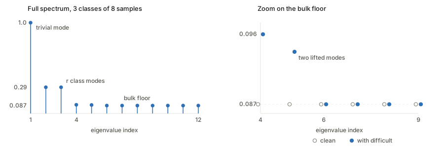
Three things follow, and they are the paper’s three claims:
- There are exactly r+1 large eigenvalues, matching r+1 classes — one trivial plus r informative — and then a cliff. Above the cliff is class structure, below it is within-class noise.
- Difficult examples inject exactly n_d extra slow modes. This is why the dimension condition in Theorem 3.4 reads r+1 \le k < n_d + r + 1: with r = 2, n_d = 2 that is k \in \{3,4\}, precisely the k for which \lambda_{k+1} lands on one of the lifted modes instead of the floor. The condition is not a technicality; it is the range of feature dimensions where the bridges bind.
- The gap closes from both sides. The floor modes rose (0.08711 \to 0.09559) and the class modes fell (0.29061 \to 0.28881). So 1 - \lambda_{k+1} shrinks from 0.91289 to 0.90441 and 4\delta/(1-\lambda_{k+1}) grows. That is Theorem 3.4.
Why the bound has this shape: 1-\lambda_{k+1} is the gap between what a rank-k approximation keeps and what it discards. A large gap means the k retained directions are decisively more informative than the dropped ones — class signal inside, noise outside, clean cut, and a linear probe finds the classes. A small gap means the (k{+}1)-th mode is nearly as important as the k-th, the truncation is arbitrary, and the representation mixes class signal with bridge structure.
Which recovers the intuition in graph terms: a difficult example is an edge between two clusters, and adding inter-cluster edges is exactly what makes a graph hard to partition. Supervised learning has labels and can use boundary points to sharpen a decision surface; unsupervised spectral clustering has none, sees a bridge, and merges across it. For the underlying spectral-graph background, see the reading a graph spectrum section of the HaoChen notes.
Results at a glance
| Setting | Bound (all of the form \tfrac{c\,\delta}{1-\lambda_{k+1}} + 8\delta) | Mechanism |
|---|---|---|
| No difficult examples (Thm 3.3) | \lambda_{k+1} = (1-\alpha)/c_2 | baseline |
| With difficult examples (Thm 3.4) | \lambda_{k+1} = \big[(1-\alpha)+r(\gamma-\beta)\big]/c_1 | strictly worse; grows with \gamma-\beta |
| Remove them (Cor. 4.1) | Thm 3.3 with n \to n-n_d | beats Thm 3.4 when \gamma-\beta > \tfrac{n_d(1-\alpha)}{nr(n-n_d)} |
| Margin tuning (Thm 4.3) | equals Thm 3.3 | subtract \bar M from \bar A |
| Temperature scaling (Thm 4.5) | Thm 3.3 inflated by 1-(n_d/n)^2+(\gamma/\beta)^2(n_d/n)^2 | multiply \bar A elementwise by T |
Note the dimension condition in Theorem 3.4: r+1 \le k < n_d + r + 1. More difficult examples widen the range of feature dimensions for which the bad bound applies.
Questions and doubts
- c_0 looks internally inconsistent. Theorem 4.3 states c_0 = (1-\alpha)+n\alpha+(n-n_d)r\beta, but solving \gamma c_2 - \beta c_1 directly gives c_2 - r\beta = (1-\alpha)+n\alpha+(n-1)r\beta. These agree only when n_d = 1. The c_1 = c_2 + r(\gamma-\beta) form already commits to one \gamma-partner per class, so (n-1) is what the stated degrees imply. Possibly a typo, possibly a different bookkeeping convention in the appendix — worth checking against the proof line by line before relying on the constant.
- The three-level model is very coarse. Real similarity matrices have structure the model cannot express: class confusability is not uniform (cats/dogs confuse more than cats/trucks), yet a single \gamma covers every difficult pair. The Wigner relaxation adds unstructured noise, which is exactly the kind of deviation that averages out — it does not test robustness to structured deviation.
- The index-matched difficult pairing is an odd modelling choice. Sample l of class i being difficult specifically with sample l of class j has no data-generating justification; it is chosen to make the Kronecker decomposition work.
- Everything is a bound comparison, not a performance comparison. The theorems compare right-hand sides. A smaller upper bound does not by itself imply smaller error, and the bounds carry the additive 8\delta which may dominate in practice.
- \alpha, \beta, \gamma are measured on trained representations, so they are outputs of the learning process, not inputs to it. Using them to explain that same process is circular unless one believes they track the underlying augmentation graph. The paper does not argue this.
- The empirical losses are not the analysed losses. Theorems 4.3/4.5 concern per-pair m_{x,x'} and \tau_{x,x'} derived from unknown constants; Eqs. 14–16 apply one global \sigma and \rho to detected pairs. The gap between prescription and implementation is never quantified.
Takeaways
- Contrastive learning trained with the spectral loss is spectral clustering of the augmentation graph. Once that is accepted, “which examples help?” becomes “which examples improve the spectral gap?” — and boundary examples worsen it by bridging clusters.
- The mechanism is intuitive in hindsight: a difficult example is an edge between two clusters, and adding inter-cluster edges is precisely what makes a graph harder to partition. Supervised learning has labels and can use such points to sharpen a boundary; unsupervised clustering has no labels and simply gets confused.
- Three interventions, three distinct matrix operations on the same target — shrink, subtract, multiply. That is a genuinely clarifying taxonomy, more so than the individual bounds.
- Practical guidance that survives the idealisation: apply a positive margin to difficult pairs, scaled by how difficult they are; use a smaller temperature on them; and if neither is available, just delete them, which is competitive whenever the difficult set is small (n_d \lesssim n^{1/2}).