Transferability and Hardness of Supervised Classification Tasks
Links
- arXiv:1908.08142 — preprint; ICCV 2019. The arXiv PDF (v1, 19 pages) carries the appendix: the full proof of Theorem 1 is Appendix A (p. 11), and the per-attribute tables the checks below use are Tables 3 and 4 (pp. 13–14).
- Interactive companion — four small experiments: type counts into a table and watch H(Y\mid Z); slide the source’s confidence and watch what the proof’s one-term drop gives away; scatter the paper’s 40 CelebA attributes against each candidate predictor; and see how far counting reads low when each source class has few images.
- Nguyen 2020 — LEEP — the direct successor, which replaces the ground-truth source labels here with a source model’s soft predictions.
- Bao 2019 — H-score — the third member of the set, approaching the same question from feature-space geometry.
- Diniz 2026 — PAS — the unsupervised counterpart: scores a source/backbone pair without any target labels, which this measure requires.
- You 2021 — LogME — the Bayesian-evidence measure, which needs only a feature extractor and so also covers regression and contrastive or language-model sources.
- Chaves 2023 — medical TE — evaluates this score on medical targets, including out-of-distribution ones.
- Claßen 2026 — TE robustness — benchmarks this measure against the others on medical imaging targets, and finds the rankings move under nothing but a change of random seed.
- Achille 2019 — task reachability — a dynamics-based view of the same question. Its static task distance is built from information stored in the weights rather than from label entropies, and it adds a factor NCE cannot see: whether fine-tuning can actually reach a good target solution from the source weights. The linked section places NCE and the other scores against the paper’s two factors.
- Runnable
code — the identity Theorem 1 turns on, the theorem itself,
the hardness bound, what H(Y\mid Z)
measures on constructed cases, a source-selection setting where dropping
the source-hardness term picks the wrong model, Figure 1 counted as
drawn, the one-term drop and a coarse-target case where it is loose, Eq.
14 without the theorem, the error window a binary target allows, the
paper’s own Tables 3 and 4, and the plug-in bias.
make verifyruns it;python3 nce.py --figuresregenerates the SVGs infigures/.
In one paragraph
Take two classification tasks over the same input instances, each with its own ground-truth label sequence — Z for the source, Y for the target. Count the joint, compute the conditional entropy H(Y\mid Z), and that number alone bounds how well a representation trained on Z will transfer to Y. The striking thing is what it does not need: no model, no features, no input data. It is solution-agnostic — two lists of labels suffice. The same quantity, applied with a trivial constant source, estimates task hardness. The catch, which the paper states and the follow-up literature then quietly drops, is that the bound has two terms: the conditional entropy and the source model’s own log-likelihood. Only when the source is held fixed does the second one disappear.
Checked against the paper’s own appendix, four things stand out. Figure 1’s “4\log 2” does not follow from the figure. The recomputed correlation for Figure 3 is 0.63, not the printed 0.78, and the target’s label entropy alone (no source) ties it on Pearson r though not on rank correlation. The case study transfers from a network that never saw the identity labels the measure counts, so it tests the statistic rather than the theorem. And the bound is tight for a one-to-one source and loose for a fine source with a coarse target.
The spine of the argument
- Define transferability as the log-likelihood on the target after freezing the source representation w_Z and retraining only the head.
- Build a classifier \bar k that composes the source model’s output with the empirical conditional \hat P(y\mid z), and assume it lives in the head space K.
- Its log-likelihood lower-bounds the best head’s. Expand it, drop all but one term inside the log, and what falls out is exactly l_Z - H(Y\mid Z).
- Hardness is transferability from a trivial task, which gives \mathrm{Hard}(T^Z)\le H(Z).
Setup and notation
| Symbol | Meaning |
|---|---|
| X=(x_1,\dots,x_n) | one input sequence, shared by both tasks |
| Y, Z | target and source label sequences over those same inputs, both ground truth |
| w_Z:\mathcal{X}\to\mathbb{R}^D | the representation learned on the source task |
| h_Z | the source head; k_Y the head retrained on the target |
| l_Z(w_Z,h_Z) | average log-likelihood of the source model on Z |
| \widetilde{\mathrm{Trf}}(T^Z\to T^Y) = l_Y(w_Z,k_Y) | transferability, Eq. 5 |
| \hat P(y,z) | empirical joint by hard counting, Eq. 6 |
| H(Y\mid Z) | the conditional entropy, Eq. 7 — the measure itself |
The setting assumption is the strong one and worth stating up front: both tasks are labelled on the same inputs. That is what makes counting \hat P(y,z) possible at all, and it is exactly what LEEP later removes.
Conditional entropy, from scratch
Before the proof, the one number it is about. Take eight images. Each has a source label z (call the two values A and B) and a target label y (0 or 1). Count how often each pair occurs:
| z= A | z= B | |
|---|---|---|
| y=0 | 3 | 1 |
| y=1 | 1 | 3 |
Look only at the images with z= A. Three of the four have y=0, so \hat P(y{=}0\mid \text{A})=\tfrac34 and \hat P(y{=}1\mid\text{A})=\tfrac14. Column B is the mirror image. The paper’s number is the average surprise of an image’s target label once its source label is known. The surprise of an event with probability q is -\ln q: zero when it is certain, large when it is rare. An image whose y is the majority one for its z has surprise -\ln\tfrac34=0.288; one that is not has -\ln\tfrac14=1.386. Six images are of the first kind and two of the second, so
H(Y\mid Z)=\frac{6\,(0.288)+2\,(1.386)}{8}=0.562\ \text{nats}.
A nat is the unit you get from the natural logarithm; a fair coin flip is \ln 2=0.693 nats. (The paper does not say which base it uses; natural logs are used throughout these notes, the code and the figures.) Without knowing z at all, y is 0 half the time and 1 half the time, so H(Y)=\ln 2=0.693. Knowing z removed 0.131 nats.
Three anchors are enough to carry the rest of the notes:
- if z determines y (each column has a single non-zero cell), H(Y\mid Z)=0;
- if z is useless (every column has the same mix), H(Y\mid Z)=H(Y), whatever z is;
- in between it is H(Y)-I(Y;Z), where the mutual information I(Y;Z) is exactly the nats that knowing z removes, 0.131 above.
Reading Eq. 7 with this in hand: \hat P(y,z) is a cell’s count over n; \hat P(z) is a column’s total over n; their ratio is \hat P(y\mid z); and the double sum adds up, over the four cells, (the cell’s share of the images) × (the surprise of its y within its column). Averaging the per-image surprises above and summing over cells are the same computation, which is the whole content of Eq. 17 in the appendix. In the interactive page, section 1 lets you edit the counts and watch each cell’s contribution.
Theorem 1, and the step it turns on
\widetilde{\mathrm{Trf}}(T^Z\to T^Y)\;\ge\; l_Z(w_Z,h_Z)\;-\;H(Y\mid Z) \tag{10}
The proof constructs a specific classifier \bar k (Eq. 9): push x through the source model to get p_Z = h_Z(w_Z(x)), then convert to a target distribution by averaging the empirical conditional against it,
p_Y(y) = \mathbb{E}_{z\sim p_Z}\big[\hat P(y\mid z)\big] = \sum_z \hat P(y\mid z)\,p_Z(z). \tag{9}
Then, assuming \bar k\in K so that l_Y(w_Z,k_Y)\ge l_Y(w_Z,\bar k),
l_Y(w_Z,\bar k) = \frac1n\sum_i\log\Big(\sum_z\hat P(y_i\mid z)P(z\mid x_i)\Big) \;\ge\; \frac1n\sum_i\log\Big(\hat P(y_i\mid z_i)P(z_i\mid x_i)\Big)
= \underbrace{\frac1n\sum_i\log\hat P(y_i\mid z_i)}_{=\,-H(Y\mid Z)} \;+\;\underbrace{\frac1n\sum_i\log P(z_i\mid x_i)}_{=\,l_Z(w_Z,h_Z)} . \tag{11–12}
Why that first term is exactly -H(Y\mid Z) — and why LEEP cannot reuse it
This is the hinge, and it is worth being precise because it resolves something left open in the LEEP notes. Because \hat P here is the hard empirical conditional,
\frac1n\sum_i\log\hat P(y_i\mid z_i) = \sum_{y,z}\hat P(y,z)\log\hat P(y\mid z) = -H(Y\mid Z)
on the nose — the code confirms it to 0.00\mathrm{e}{+}00. The step closes because \frac1n\sum_i\log Q(y_i\mid z_i) is maximised over conditionals Q by precisely that \hat P.
LEEP runs the same argument with a soft conditional built from a source model’s softmax. The identity then fails in the wrong direction — the soft conditional is dominated by the hard one, measured at 0.138 nats below on the same data — so the one-term-drop lands strictly below NCE and cannot establish LEEP’s Property 2. That property still holds empirically, but by a route this proof does not supply.
Checking the theorem honestly
The bound is stated for a head space K that contains \bar k, and the paper’s Discussion 2 says how to arrange that: take K = K'\cup\{\bar k\} and pick whichever scores better. That assumption is load-bearing. Checking the bound against a plain linear head on the frozen representation — a K that does not contain \bar k — produces violations, and they are the checker’s fault, not the theorem’s. Done correctly:
| alignment | l_Z | H(Y\mid Z) | bound | actual Trf | holds |
|---|---|---|---|---|---|
| 0.3 | −0.0097 | 1.3355 | −1.3452 | −1.3357 | yes |
| 1.0 | −0.0313 | 1.1113 | −1.1425 | −1.1145 | yes |
| 2.0 | −0.0378 | 1.0104 | −1.0482 | −1.0204 | yes |
| 4.0 | −0.0069 | 0.2827 | −0.2896 | −0.2875 | yes |
Tight throughout in this family, where the source is confident about its own labels (l_Z\approx 0) and Y becomes more nearly a one-to-one function of Z as the alignment grows. The next two subsections say where that tightness comes from and where it stops.
The appendix proof, line by line
Appendix A (p. 11 of the arXiv PDF) has four moves, and only the third is an inequality that loses anything:
- The best head beats \bar k. \widetilde{\mathrm{Trf}}=l_Y(w_Z,k_Y)\ge l_Y(w_Z,\bar k), because k_Y is the best head in K and the assumption is that \bar k\in K. No loss here if \bar k really is one of the candidates; a hard assumption if it is not.
- Build \bar k. For an image x_i its probability of the true target label y_i is \sum_z \hat P(y_i\mid z)\,p(z\mid x_i): ask the source model how likely each source label is, and for each one look up how often that source label goes with y_i in the counted table.
- Replace the sum by one of its terms. Every term is non-negative, so the sum is at least the z=z_i term alone, and \log is increasing. This is Eq. 11 and it is where the bound is paid.
- Split the log of a product. \log\big(\hat P(y_i\mid z_i)\,p(z_i\mid x_i)\big) is a sum of two logs. Averaged over i, the second is l_Z by definition and the first is -H(Y\mid Z) by grouping the images by their (y,z) pair and counting (Eq. 17), exactly as in the eight-image example.
What the one-term drop gives away
Step 3 costs, for image i,
\ln\!\Big(1+\frac{\sum_{z\ne z_i}\hat P(y_i\mid z)\,p(z\mid x_i)}{\hat P(y_i\mid z_i)\,p(z_i\mid x_i)}\Big)\ \ge 0 ,
the log of (the whole sum) over (the kept term). It is zero in two cases: the source is certain of z_i, or y_i never occurs with any other source label. Otherwise there is a second term to throw away. Six points make it concrete: Z=(0,0,0,1,1,1), Y=(0,0,1,1,2,2), and a source that puts probability c on the right z and 1-c on the other:
| c | l_Z | l_Y(\bar k) | bound l_Z-H | gap |
|---|---|---|---|---|
| 0.500 | −0.6931 | −1.0986 | −1.3297 | 0.2310 |
| 0.800 | −0.2231 | −0.7853 | −0.8597 | 0.0744 |
| 0.950 | −0.0513 | −0.6707 | −0.6878 | 0.0171 |
| 0.999 | −0.0010 | −0.6372 | −0.6375 | 0.0003 |
Here H(Y\mid Z)=0.6365, and the gap is exactly \tfrac13\ln(1/c) in every row. The \tfrac13 is the fraction of points, the two with y=1, whose label is possible under both source classes; the four others have a single term and lose nothing.
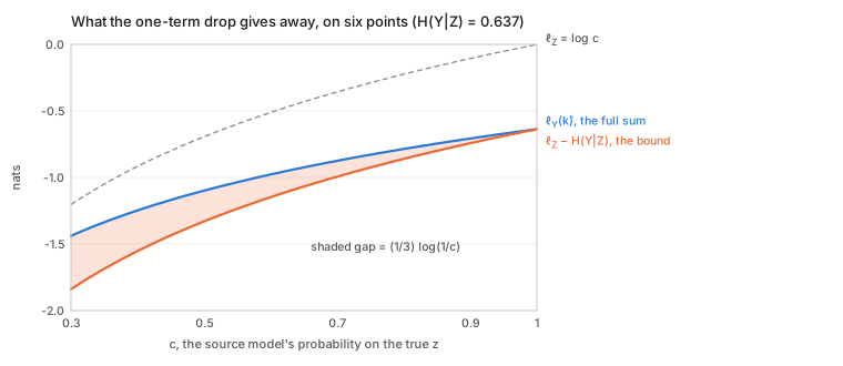
The gap does not care whether the confusion matters to the target. Let Z have 2g classes and Y=Z\,//\,g, a coarse target of which Z is a refinement, so H(Y\mid Z)=0. A source that is sure of the group but spreads its probability over the g classes inside it has l_Z=-\ln g. The target log-likelihood of \bar k is exactly 0 (all the mass sits on the right group), and the bound is -\ln g:
| g | l_Z | H(Y\mid Z) | bound | l_Y(\bar k) | gap |
|---|---|---|---|---|---|
| 1 | 0 | 0 | 0 | 0 | 0 |
| 2 | −0.6931 | 0 | −0.6931 | 0 | 0.6931 |
| 4 | −1.3863 | 0 | −1.3863 | 0 | 1.3863 |
| 8 | −2.0794 | 0 | −2.0794 | 0 | 2.0794 |
So the bound is tight for a one-to-one source and can be arbitrarily loose for a fine source and a coarse target: it charges the target for every distinction the source cannot make, though the target never asked for one. Something like a 1000-way source and a dog-or-not target is this case.
What H(Y\mid Z) actually measures
Three regimes, all exact in the code:
| case | H(Y\mid Z) | |
|---|---|---|
| Z bijective with Y | 0.0000 | nothing left to learn; transfer is free |
| each Z class splits into 2 | 0.6931 | \log 2 |
| each Z class splits into 4 | 1.3863 | \log 4 |
| Z trivial, \lvert\mathcal{Y}\rvert=4 | 1.3863 | =H(Y) |
| Z trivial, \lvert\mathcal{Y}\rvert=16 | 2.7726 | =H(Y)=4\log 2 |
A trivial source gives H(Y\mid Z)=H(Y) — there is nothing to condition on, so the transfer must supply all of the information. The measure is, straightforwardly, how much information about Y is still missing once you know Z.
Figure 1 counted as drawn
The paper illustrates this with five toy panels (its Figure 1) and says, in Sec. 3.3, that (c) has H(Y\mid Z)=0, (d) and (e) have \log 2, and (a) and (b) have 4\log 2, “the highest CE”, so that transfer is hardest for them. Counting the panels as drawn (eight examples each, equal runs) gives something different:
| panel | source Z | target Y | \lvert\mathcal Y\rvert | H(Y) | H(Y\mid Z) | I(Y;Z) | text says |
|---|---|---|---|---|---|---|---|
| (a) | constant | two halves | 2 | 0.693 | 0.693 | 0 | 4\log 2 |
| (b) | constant | alternating | 2 | 0.693 | 0.693 | 0 | 4\log 2 |
| (c) | two halves | same halves, relabelled | 2 | 0.693 | 0 | 0.693 | 0 |
| (d) | two halves | alternating | 2 | 0.693 | 0.693 | 0 | \log 2 |
| (e) | two halves | four levels | 4 | 1.386 | 0.693 | 0.693 | \log 2 |
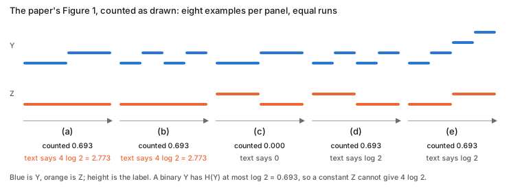
The text itself says T^Y is binary in (a–d). A binary target has H(Y)\le\log 2, and a constant source leaves H(Y\mid Z)=H(Y), so (a) and (b) cannot be 4\log 2=\log 16; that value needs sixteen balanced target labels. As drawn, (a), (b), (d) and (e) all tie at \log 2 and only (c) differs, so the figure does not show the ordering the paragraph reads off it. The tie is not an accident: (a), (b) and (d) all have I(Y;Z)=0, because in (d) each source class contains one half-run of each target label, which is as uninformative as a constant source. Panel (e) reaches \log 2 by another route, \ln 4 of target entropy minus the \ln 2 the source supplies. This looks like a slip in the caption arithmetic and not in the theory. The 16-class row in the table above shows what would give 4\log 2, but the figure has two labels.
Task hardness
Hardness is the optimal loss, \mathrm{Hard}(T^Z)=\min_{w,h}\mathcal{L}_Z(w,h)=-l_Z(w_Z,h_Z) (Eq. 13). Applying Theorem 1 with a trivial constant source C gives
\mathrm{Hard}(T^Z)\;\le\;H(Z\mid C) \tag{14}
and since conditioning on a constant is no conditioning at all, H(Z\mid C)=H(Z) — the plain label entropy. So the paper’s hardness estimate is, after unwinding, the entropy of the source label distribution. Verified across \lvert\mathcal{Z}\rvert\in\{2,4,8,16\}: H(Z\mid C) and H(Z) agree to four decimals and the bound holds every time.
That is a genuinely cheap estimator and it correlates well in their experiments. It is also worth seeing plainly for what it is: a task with more, more balanced labels is estimated as harder, with no reference to the inputs. The paper concedes the point — “this result does not imply that the input domain has no impact on task hardness; only that the distribution of training labels already provides a strong predictor” — but the estimator cannot distinguish a 4-class problem that is trivially separable from a 4-class problem that is not.
Eq. 14 also needs no theorem. A head that ignores x and always outputs the label frequencies \hat P(z) has training cross-entropy exactly -\frac1n\sum_i\log\hat P(z_i)=H(Z), and any model class that can output a bias can do that, so \mathrm{Hard}(T^Z)=\min L_Z\le H(Z) follows in one line. The code checks it (for \lvert\mathcal Z\rvert=2,5,16 the frequency predictor’s loss is 0.6931,\ 1.6091,\ 2.7717, equal to H(Z), and 2000 random rival input-blind predictors never beat it). So the “hardness estimate” is the loss of the predictor that has learned nothing, an upper bound that is loose by however much the inputs help.
The term the later papers drop
Theorem 1 has two terms, and this matters more than it looks.
The paper’s own stated use is: fix the source, and then l_Z(w_Z,h_Z) is a constant, so ranking multiple targets by -H(Y\mid Z) alone is licensed. Explicitly: “when the source task T^Z is fixed, the log-likelihood l_Z(w_Z,h_Z) is a constant. In this case, the transferability only depends on the CE H(Y\mid Z).”
But NCE is subsequently used — by LEEP, by H-score, and as a baseline generally — for source selection: fixed target, varying source. There l_Z is not constant, and dropping it is an extra, unstated assumption.
Whether it bites depends on whether the two terms move together. Varying them independently — how noisily x carries Z (which drives l_Z) against how tightly Y follows Z (which drives H(Y\mid Z)) — they come apart:
| source | l_Z | H(Y\mid Z) | -H(Y\mid Z) | l_Z-H | actual Trf |
|---|---|---|---|---|---|
| clean x, loose Y\mid Z | −0.4985 | 1.1940 | −1.1940 | −1.6925 | −1.2562 |
| clean x, tight Y\mid Z | −0.5049 | 0.4891 | −0.4891 | −0.9940 | −0.6710 |
| noisy x, tight Y\mid Z | −1.3592 | 0.6126 | −0.6126 | −1.9718 | −1.1275 |
| noisy x, loose Y\mid Z | −1.3637 | 1.1254 | −1.1254 | −2.4891 | −1.2914 |
| v. noisy x, tight Y\mid Z | −1.3633 | 0.2004 | −0.2004 | −1.5637 | −0.9732 |
Spearman against actual transfer: -H(Y\mid Z) gives +0.800, the full l_Z-H(Y\mid Z) gives +0.900. And NCE’s top pick is the wrong source — it prefers the very noisy one on the strength of its low conditional entropy, while the clean source with looser alignment actually transfers best. The reason is structural: training on an unpredictable Z yields a representation that learned nothing, and H(Y\mid Z) cannot see that, because it never looks at x. Solution-agnosticism is the selling point and the blind spot at once.
To be fair about the strength of this: where source hardness and label alignment do move together — which is common, since a source with many fine-grained classes tends to be both harder and more informative — a generator varying them in step shows no disagreement at all. The assumption is real, it is unstated, and it is satisfied often enough that NCE works in practice.
Restoring l_Z is not a free fix either. The coarse-target table earlier shows the term charging a target for the source’s own confusion inside a group of source classes that the target does not distinguish. Both terms of the bound are honest lower-bound pieces; neither is a clean measure of how well a representation will carry over.
Does the evidence show what the paper says it does?
The experiments (Sec. 5) never evaluate Theorem 1’s inequality. They plot the counted H(Y\mid Z) against the test error of a linear SVM on frozen features (Figures 2 and 3), and the counted H(Z) against the test error of a network trained from scratch (Figure 6). The theorem is a statement about training log-likelihood and a head that may be \bar k; Definition 1 is about accuracy and Eq. 5 replaces it, under a stated non-overfitting assumption, with the training log-likelihood; Sec. 5 then says outright that test accuracy is “generally more important” and reports that. What the figures test is the weaker claim that the counted number predicts the error. Tables 3 and 4 of the appendix list, for all 40 CelebA attributes, the conditional entropy given identity, the attribute’s own entropy H(Y) (which is the “hardness” of Eq. 14) and the linear SVM’s accuracy from identity features. That is enough to recompute the claim.
A binary target squeezes the error into a window
For a binary target there is a short argument for why some correlation must appear. Consider the best guesser that sees only z: within each source class it says the majority target label. Its error is P_e=\sum_z\hat P(z)\min(q_z,1-q_z) with q_z=\hat P(y{=}1\mid z), and H(Y\mid Z)=\sum_z\hat P(z)\,h(q_z) with h the binary entropy. Two facts about h bracket P_e:
- h is concave, so by Jensen H(Y\mid Z)\le h(P_e), i.e. P_e\ge h^{-1}\!\big(H(Y\mid Z)\big);
- h(q)\ge 2\ln 2\cdot\min(q,1-q) (a concave function above its chord), so P_e\le H(Y\mid Z)/(2\ln 2).
Both ends are attained (one source class with q=0.1 hits the lower end; half the mass at q=\tfrac12 and the rest at q=0 hits the upper end), and 2000 random tables never leave the window. At H(Y\mid Z)=0.3 the window is [0.089,\,0.216], and its top is 2.4\times its bottom. So across binary targets the counted number pins the ideal error to a band, and a correlation with the error of a decent classifier is close to arithmetic.
What the paper’s own tables give
Recomputing from Table 3 (rows 9 and 11) and Table 4, for the 40 CelebA attributes:
| Pearson r | Spearman \rho | |
|---|---|---|
| CE =H(Y\mid\text{ID}) against transfer error | 0.630 (Fig. 3 prints 0.78) | 0.825 |
| same, without Big Lips | 0.726 | |
| H(Y), the label entropy alone, against transfer error | 0.621 | 0.660 |
| CE against dedicated-network error | 0.525 | |
| H(Y) against dedicated-network error | 0.581 (Fig. 6a prints 0.58) | |
| \mathrm{CE}/H(Y) against transfer error | 0.333 | |
| partial r of CE with error, given H(Y) | 0.326 | |
| partial r of H(Y) with error, given CE | 0.299 |
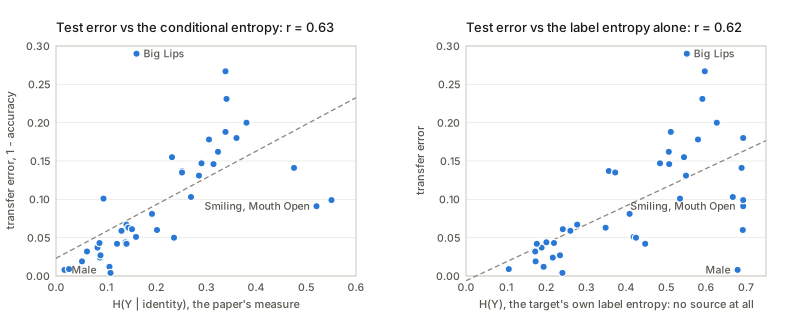
Figure 6(a)’s printed 0.58 reproduces to the third digit, which says the tables and the transcription are consistent, and makes the mismatch for Figure 3 (0.63 against 0.78) a real discrepancy and not a typing error. Removing Big Lips gets to 0.73 but no further; I cannot tell whether the figure used unrounded values or a different split. Two things then matter for what the correlation means:
- The label entropy alone ties it on Pearson. H(Y) uses no source at all and reaches 0.62 against 0.63. The paper reports only Pearson. On rank correlation the conditional entropy is clearly ahead (0.83 against 0.66), and each still explains something after controlling for the other (partial 0.33 and 0.30). So the conditional entropy does carry signal beyond the target’s base rate, and a good part of the headline correlation is what the base rate gives free.
- Rare attributes look transferable for free. A rare attribute has small H(Y), so its conditional entropy is small whatever the source says. Pale Skin ranks 12th of 40 by CE, yet the SVM’s error (0.042) equals the error of always answering “no” (0.043). Big Lips is the opposite: a middling CE and the worst transfer error in the table:
| attribute | CE | H(Y) | CE/H(Y) | always-majority error | SVM error |
|---|---|---|---|---|---|
| Male | 0.017 | 0.679 | 0.03 | 0.416 | 0.008 |
| Bald | 0.026 | 0.107 | 0.24 | 0.022 | 0.009 |
| Pale Skin | 0.122 | 0.177 | 0.69 | 0.043 | 0.042 |
| Blurry | 0.139 | 0.201 | 0.69 | 0.051 | 0.044 |
| Big Lips | 0.161 | 0.552 | 0.29 | 0.241 | 0.290 |
| Smiling | 0.521 | 0.693 | 0.75 | 0.491 | 0.091 |
| Mouth Open | 0.551 | 0.693 | 0.80 | 0.491 | 0.099 |
(“Always-majority error” is the rarer class’s rate, recovered from H(Y); it assumes the tables report plain accuracy, which the paper does not say. If they are class-balanced accuracies, this column and the window below change meaning, though the correlations above do not.) Male is the clearest positive case: the measure cuts a large H(Y)=0.679 to 3\% of itself, so it plainly can see an identity-determined attribute. Against the fraction \mathrm{CE}/H(Y) that identity leaves unexplained the correlation with error falls to 0.33: the raw correlation is partly a level effect, and the ratio is the version that isolates what the source contributes.
The printed correlations are also a selected sample. The twelve panels in the main-text Figure 2 have r=0.92–0.97. The appendix shows the whole grid: for all 40 CelebA source attributes r runs from 0.73 to 0.94 (mean 0.84), and the four CelebA panels chosen for the main text (source attributes 18, 20, 26 and 36) are exactly the four highest of the forty. The 85 AwA2 sources run 0.91–0.98 (mean 0.95). The identity source’s printed 0.78 is inside the CelebA range, with 35 of the 40 binary sources above it.
The window, against the SVM’s error
Putting the 40 SVM errors against the window [h^{-1}(\mathrm{CE}),\ \mathrm{CE}/(2\ln 2)] that a guesser seeing only the identity could reach:
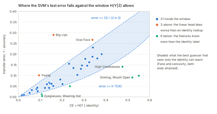
- 31 inside, so for most attributes the error is what the identity table allows.
- 3 above (Big Lips, Oval Face, Young): the linear head does worse than a lookup on the identity label would. That is what the \bar k\in K condition failing looks like: the counted table is usable only by a head that can consult the source’s softmax over identities, and a linear SVM cannot. (Sampling noise between the training table and the test error could also account for Oval Face, which is borderline once the bias below is allowed for.)
- 6 below (Smiling, Mouth Open, High Cheekbones, Eyeglasses, Wearing Hat, Bangs): the frozen features do better than any guesser that knows only the identity could. For Smiling and Mouth Open the window starts at 0.215 and 0.240 and the SVM gets 0.091 and 0.099. The representation encodes expression the identity label does not. This is the cleanest evidence that a label-only number describes Z, not what the network learned, and it is the gap that the feature-space scores (H-score, LogME) exist to close.
The estimator is biased low, and by about the size of the smallest values
H(Y\mid Z) is computed by splitting the images by source label and measuring the mix of y inside each group. A small group looks purer than its truth by chance. With CelebA’s 182{,}626 training images over 10{,}177 identities there are 17.9 images per identity, and even for an attribute independent of identity the counted value falls short of the truth by about (|\mathcal Y|-1)\,|\mathcal Z|/(2n)=0.028 nats (exact binomial expectation and a full Monte Carlo agree):
| P(y{=}1) | true H(Y\mid Z)=H(Y) | counted, exact | shortfall | Monte Carlo |
|---|---|---|---|---|
| 0.022 | 0.1057 | 0.0794 | 0.0264 | 0.0787 |
| 0.100 | 0.3251 | 0.2930 | 0.0321 | 0.2921 |
| 0.240 | 0.5511 | 0.5217 | 0.0294 | 0.5212 |
| 0.500 | 0.6931 | 0.6644 | 0.0287 | 0.6647 |
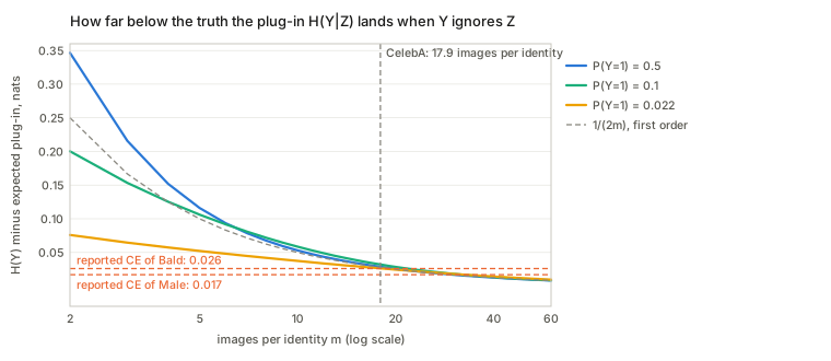
The paper’s smallest reported values are 0.017 (Male) and 0.026 (Bald), below the bias itself. The order among the top few attributes is inside the estimator’s own error. And the effect scales with the number of source classes: a source with as many labels as images reads 0 for every target, so the measure rewards fine-grained sources by construction. Against a noise-only baseline the reported CE is 0.84 of what pure noise would give for Pale Skin, 0.83 for Mouth Open and 0.82 for Blurry, so for those the identity labels tell the counting almost nothing; Male is 0.03. (The bias also lifts the window a little. Adding 0.028 to each CE moves the top end for Young from 0.069 to 0.089 against an error of 0.101, for Big Lips from 0.116 to 0.136 against 0.290, and for Oval Face from 0.245 to 0.265 against 0.267; Young and Big Lips stay above, and Oval Face becomes a borderline case.)
What is transferred in the case study
For the Figure 2 experiments each source is a binary attribute and a ResNet-18 is trained on it, so the source premise of Theorem 1 holds, but the head is a linear SVM, so \bar k\notin K. For the face-recognition case study (Sec. 5.2, Table 1, Figure 3) the counted Z is CelebA’s identity label, but the network that is transferred is a ResNet-101 trained on MS-Celeb-1M and VGGFace2 “following removal of subjects included in CelebA”. It never saw the labels the measure counts, so the setting of Theorem 1 (the same Z for the model and for the table) is not met there either. That is a fair transfer experiment and not a test of the theorem, and its printed correlation (0.78, which recomputes to 0.63) is below the AwA2 range and within the CelebA one.
How the three measures relate
| NCE (this paper) | LEEP | H-score | |
|---|---|---|---|
| what it reads | two ground-truth label sequences | source model’s softmax \theta(x) | penultimate features h(x) |
| needs a trained source model | no (for the measure) | yes | yes |
| needs source labels on target inputs | yes | no | no |
| the head | \hat P(y\mid z), hard counting | \hat P(y\mid z), soft counting | optimal linear head, eliminated |
| what it estimates | a lower bound, with a second term | a lower bound at one head | a second-order approximation to the supremum |
| assumption | shared input instances | source labels code the target | weak dependence, o(\varepsilon^2) |
The lineage is clean. NCE needs the source labels but no model; LEEP needs the model but no source labels — it replaces the ground-truth z_i with the source model’s prediction, and that single substitution is the entire difference. H-score comes at the same target from the other side, working in feature space and optimising the head away rather than constructing one. Read the three together and the design space is essentially: which representation do you read (labels, softmax, features), and do you evaluate one head or the best one?
Questions and doubts
- The measure is model-free; the bound is not. H(Y\mid Z) needs only labels, which is the headline. But Theorem 1’s right-hand side contains l_Z(w_Z,h_Z), which requires a trained source model. The advertised cheapness belongs to the measure alone, and only survives to the bound when the source is fixed.
- The \bar k\in K assumption is load-bearing and easy to miss. Check the bound against a head space that excludes \bar k and it fails; the paper handles this in a Discussion paragraph rather than in the theorem statement.
- Source selection is outside what is licensed, as the table above shows. Every later paper that benchmarks against NCE uses it in exactly that regime.
- Hardness reduces to label entropy. Eq. 14 unwinds to \mathrm{Hard}(T^Z)\le H(Z), the loss of the predictor that ignores the input, so the estimator cannot separate two tasks with the same label distribution and different intrinsic difficulty. The correlations reported are real but the mechanism is blunter than “hardness” suggests. The CelebA one recomputes to 0.581, the weakest of the three data sets (0.58, 0.82, 0.96).
- Figure 1’s “4\log 2” does not follow from the figure. The text says T^Y is binary in panels (a–d), and a binary target cannot have H(Y\mid Z) above \log 2; counted as drawn, (a), (b), (d) and (e) all tie at \log 2. The ordering the paragraph reads off the figure is not in it. I read this as a caption slip and not a flaw in the idea, but the toy example is the paper’s only intuition for why a trivial source is hardest.
- Figure 3’s printed correlation does not reproduce. r=0.78 is printed; Tables 3 and 4 give 0.63 (0.73 without Big Lips; Spearman 0.83). The same recomputation reproduces Figure 6(a)’s 0.58 to the third digit, so this is not a transcription problem. I do not know whether the figure used unrounded values, a different split or a different error.
- The label entropy alone ties the headline correlation. H(Y), with no source, gives Pearson 0.62 against the conditional entropy’s 0.63; on rank correlation the conditional entropy is clearly ahead (0.83 against 0.66). The paper reports only Pearson and never compares with a base-rate predictor, so how much of the “remarkable” correlation is transfer and how much is the target’s base rate is not shown. The conditional entropy does carry signal beyond it (partial r\approx0.3).
- The printed correlations are a selected sample. The four CelebA panels in the main-text Figure 2 are exactly the four highest of the forty in the appendix (0.93–0.94, against a mean of 0.84 over all forty).
- The experiments do not test Theorem 1. They compare the counted number with the test error of a linear SVM (hinge loss, \bar k\notin K), not with the log-likelihood the theorem bounds. In the case study the transferred network was trained on other identities, not on the labels that are counted. The bound itself is checked in the code, and it holds, but only there.
- The bound is tight for a bijection and loose for a coarse target. The one-term drop costs \ln(1+\text{other terms}/\text{kept term}) per image. For a fine source and a coarse target it charges the target the source’s whole within-group confusion (\ln g for g classes), so the bound can be arbitrarily far below the truth exactly where the transfer is easy.
- The counted H(Y\mid Z) is biased low, by about the size of its smallest values. With 17.9 images per identity the shortfall is about 0.028 nats even for an attribute independent of identity, against reported values of 0.017 and 0.026 for Male and Bald. It falls to 0 as the source gets as many labels as images, so a fine-grained source looks informative by construction. A bias-corrected version (Miller–Madow, or a shrinkage estimator) would be the natural repair, and the paper does not raise it.
- A label-only number describes Z, not the representation. On the plain-accuracy reading, six attributes (Smiling, Mouth Open, High Cheekbones, Eyeglasses, Wearing Hat, Bangs) transfer better than any guesser that sees only the identity could, and three (Big Lips, Oval Face, Young) transfer worse than a lookup would. Feature-space scores see the first group; only a head that can consult the source’s softmax could use the counted table in the second.
- Rare attributes look transferable for free. Pale Skin ranks 12th of 40 by conditional entropy and its SVM error equals that of always answering “no”.
- Plain or class-balanced accuracy? The tables say “accuracy” and the paper does not say which. The correlations do not depend on it; the always-majority baseline and the window do.
- Shared input instances is a strong setting assumption, and the one the paper is most candid about — the conclusion flags extending beyond it as future work. LEEP’s main contribution is removing it.
- Everything is empirical log-likelihood on the training set, justified by “the non-overfitting assumption holds even for large networks”. Discussion 3 sketches a McDiarmid route to the expected log-likelihood but does not carry it out.
Takeaways
- The measure is two lists of labels and a counting argument. That it predicts transfer at all — no model, no features, no inputs — is the surprising result, and it is why this paper seeded the two that followed.
- H(Y\mid Z) is how much about Y is still missing once you know Z. A bijective source gives zero, a trivial source gives H(Y), a k-way split gives \log k. Nothing subtler is going on.
- The hinge identity is that the hard empirical conditional makes the counting exact: the average of \log\hat P(y_i\mid z_i) is -H(Y\mid Z). That is why this proof lands on a clean number and why LEEP’s soft version cannot inherit it — the cleanest thing to carry between the two papers. The one-term drop before it is a separate step, and it is the one that loses.
- Read Theorem 1’s two terms, not one. The paper is explicit that dropping l_Z requires a fixed source; the field then used it for source selection anyway. Where source hardness and label alignment happen to move together that is harmless, and where they do not, NCE picks the wrong model.
- Its correlation with error is partly the target’s base rate. For a binary target the counted number pins the ideal error to a window [h^{-1}(H),\,H/(2\ln 2)], and in the paper’s own tables the label entropy H(Y) alone ties the conditional entropy on Pearson r (0.62 against 0.63, with the paper’s printed 0.78 not reproducing). The conditional entropy still leads on rank correlation, so it is a real signal on top of the base rate, just a smaller one than it looks.
- Two things to fix before trusting small differences. The counted value is biased low by about 0.028 nats at 17.9 images per class, as large as the top of the ranking, and the bound charges a coarse target for a fine source’s confusions. The idea survives both; the small differences among the top-ranked attributes do not.