The Lagrange multiplier: the best point on a trail, and what the rule costs

Links

• Source of the story: YouTube video on the Lagrange multiplier. The hiking trail, the contour-map argument, the fence by the river, shadow prices, the bead on a wire, the box of gas and the list of limits all follow that video. They are retold here in my own words from its transcript. The tangency figure, the maximum-entropy die and the \theta–\eta figure are my additions, linking the idea to exponential families.
• Interactive companion: six widgets: walk a hiker along the trail, the before/at/after snapshots, slide along a line to a circle, resize the fenced field and its budget, tilt a die under a mean constraint, and move between \theta and \eta.
• Fisher information: the slope of the \theta–\eta curve at the end.
• Dually flat structure (Amari): where the pair (\theta,\eta) becomes the two coordinate systems of the geometry.

In one paragraph

Many problems ask for the best value of a quantity F while obeying a rule G=c: the highest point you can reach on a trail, the most area from a fixed length of fence, the distribution of most entropy with a fixed average. Setting the derivative of F to zero is the wrong test, because the best point on the trail is usually not flat ground. The right test is geometric. At the best point the trail touches a contour line of F without crossing it, so the two gradients lie on one line: \nabla F=\lambda\nabla G. The factor \lambda, the Lagrange multiplier, is more than bookkeeping. It is the price of the rule: how fast the best achievable value changes when the rule is loosened.

The question: the best point on a trail

You hike along a trail on a mountainside and want the highest point you will reach while staying on it. The summit does not help, since the trail never goes there. This is a different question from “where is the top of the mountain”.

The usual move, looking for flat ground, fails here. The best point on the trail is generally not flat ground, and the slope may still point uphill right where you stand: you would keep climbing if the trail let you.

Call the quantity to maximise F (the height) and write the trail as G(x,y)=c. Substituting the rule into F and differentiating is possible for easy rules, but a circle is not a single function of x, many rules cannot be solved for either variable, and with ten variables and three rules the substitutions become a problem of their own. The picture below avoids solving the rule at all.

The map picture: the trail must touch a contour

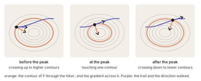
A contour line is a curve of constant height, so walking along it goes neither up nor down. The gradient \nabla F is the steepest-uphill direction, and because moving along a contour changes nothing, it points straight across the contour, perpendicular to it.

Now draw the trail on the same map. At first it cuts across one contour after another, each higher than the last: you are still climbing. After the peak it crosses them the other way: you descend. At the highest point it is not crossing at all. It touches one contour and turns away.

At the best point, the trail and a contour of F are tangent.

If the trail still crossed a contour there, one direction along it would reach a higher one, so you would not yet be at the maximum. The three panels above are the same trail at three moments, with the hiker’s own contour in orange. (The interactive page lets you walk the trail and watch the arrows.)

From tangent curves to one equation

• \nabla F is perpendicular to F’s contour.
• The trail is itself a contour of G (every point on it gives G the same value), so \nabla G is perpendicular to the trail.
• Tangent curves have parallel normals. So at the best point the two gradients lie on one line. They need not have the same length, so one is a multiple of the other:

\nabla F=\lambda\,\nabla G .

In two dimensions this is two equations, one per component, plus the rule G=c itself: three equations for three unknowns x,y,\lambda.

The same thing packages into one function, the Lagrangian,

\mathcal L(x,y,\lambda)=F(x,y)-\lambda\big(G(x,y)-c\big).

Setting every partial derivative of \mathcal L to zero gives exactly those three equations; \partial\mathcal L/\partial\lambda=0 just re-imposes the rule. One extra unknown turns a constrained problem into an unconstrained one.

Why the condition is right. Stand on the trail and take a small allowed step d. It keeps G unchanged, so d\perp\nabla G. At the best point F must not change for any such step, so \nabla F has no component along the allowed directions, so it is parallel to \nabla G.

A first concrete example: the nearest point on a line

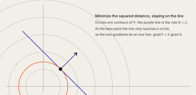
Find the point on the line x+y=c closest to the origin. Here F=x^2+y^2 (squared distance), whose contours are circles around the origin, and the rule is G=x+y=c. Slide along the line: the circle through your point shrinks, then grows. At the turning point the line only touches a circle, \nabla F points straight away from the origin and \nabla G=(1,1) is perpendicular to the line, and the two are parallel. Solving \nabla F=\lambda\nabla G gives x=y, and the rule then places the point at x=y=c/2. The interactive page has a slider for the point and one for c.

The fence by the river, and what \lambda really means

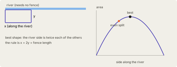
You have 40 m of fencing and want to enclose a rectangular field with a straight river as one side. Let x be the side along the river and y each of the other two sides. The area is F=xy and the rule is G=x+2y=40.

• \nabla F=(y,\,x): making x longer adds a strip of width y, making y longer adds a strip of length x.
• \nabla G=(1,\,2): a metre of x costs one metre of fence, a metre of y costs two.
• Parallel gradients give y=\lambda and x=2\lambda. Back in the rule, 4\lambda=40, so \lambda=10, y=10 m, x=20 m. The river side is twice each of the others.

Sharing the fence evenly over three sides (about 13.3 m each) gives roughly 178 m². The Lagrange shape gives 200 m². The “even split” is not best because one side needs no fence.

The multiplier came out as 10. Now give yourself 41 m instead of 40. The best area rises by a little more than 10 m². That match is the point.

Why \lambda is a price. Loosen the rule slightly. As the best point moves, F changes by \nabla F\cdot(\text{move}), and at the optimum \nabla F=\lambda\nabla G. So whatever change the move makes in G, it makes \lambda times as much in F. And the change in G is exactly how far you loosened the rule. So the best achievable value F^*(c) obeys

\frac{dF^*}{dc}=\lambda .

(For the fence the best area is F^*(L)=L^2/8, whose slope L/4 is exactly the y we found, which is \lambda. At 40 m that slope is 10. Going from 40 to 41 m adds slightly more than the slope at 40, because the slope itself is still growing along the way.)

Shadow prices. An economist reads the same fact as: for a company maximising profit under a fixed budget, the multiplier on the budget is the extra maximum profit from one more dollar. A multiplier of 1.3 means a dollar more is worth about $1.30. It never appears on an invoice, hence “shadow price”.

A bead on a wire. Gravity pulls the bead down and the wire must push back to keep it on its path. Write the wire as a rule and the multiplier is the force the wire exerts, without modelling the wire.

The general statement

Optimise f(x), x\in\mathbb R^n, subject to rules g_1(x)=\dots=g_m(x)=0. Stationary points of

\mathcal L(x,\lambda)=f(x)-\sum_i\lambda_i g_i(x)

satisfy \nabla f=\sum_i\lambda_i\nabla g_i and all g_i=0. The gradient of f must lie in the span of the rule normals: no allowed direction is left to improve in. With one rule and two unknowns this is the tangent-contour picture; with more rules it is the same statement in more dimensions. The price reading carries over, with one price \lambda_i per rule: \partial f^*/\partial c_i=\lambda_i (the envelope theorem).

Maximum entropy: a box of gas, and a die

Take a box of gas whose molecules share a fixed total energy. Among all ways to spread probability over the states, take the one of greatest entropy, subject to two rules: the probabilities sum to 1, and the average energy is fixed. Two rules give two multipliers, and the answer is the Boltzmann distribution: the probability of a state falls exponentially with its energy.

The multiplier on the energy rule is 1/(kT). By the price reading it measures how much extra maximum entropy one more unit of energy buys. That also explains the direction of heat flow. Give a unit of energy to a cold object and its entropy rises a lot; take it from a hot one and its entropy falls less. The total rises, so heat flows from hot to cold.

A die is the same problem in miniature. Maximise H(p)=-\sum_i p_i\log p_i subject to \sum_i p_i=1 and \sum_i i\,p_i=m. The Lagrangian carries one multiplier per rule:

\mathcal L=H(p)-\alpha\Big(\sum_i p_i-1\Big)-\lambda\Big(\sum_i i\,p_i-m\Big).

Setting \partial\mathcal L/\partial p_i=0 gives -\log p_i-1=\alpha+\lambda i, hence

p_i\;\propto\;e^{-\lambda i}.

This is an exponential family. The multiplier is the natural parameter (with a sign), and the quantity you constrained, here the roll value, is the sufficient statistic. Several constrained averages E[T_k] give p\propto\exp\!\big(\sum_k\lambda_kT_k\big).

A required mean of 3.5 is what a fair die already has, so the rule costs nothing: \lambda=0 and the bars are flat. Force the mean away from 3.5 and the weight tilts exponentially to one end, and \lambda is the price of that pull. (In the interactive page, slide the required average.)

\theta and \eta: two addresses for one distribution

Write the die family as p_\theta(i)\propto e^{\theta i}, so \theta=-\lambda. Let \psi(\theta)=\log\sum_i e^{\theta i} be the log of the normaliser. Then the expected roll is \eta=\psi'(\theta) and its variance is \psi''(\theta). Each \theta gives one \eta and each \eta gives one \theta, because \psi''>0 makes the curve monotone: they are two addresses for the same distribution.

The slope of that curve is the variance, which is the Fisher information. Where the curve is steep (near \theta=0), a small change in \theta moves the average a lot; near the ends the weight is already piled onto one face and extra tilt barely moves it.

The price relation reads in both directions. Moving the constraint value \eta changes the best entropy at rate -\theta (equivalently \lambda), and moving \theta changes the log-normaliser \psi at rate \eta. The two potentials are Legendre duals, and this curve is the bridge between them. This is the pair (\theta,\eta) of the dually flat structure: the multipliers are the natural coordinates and the constrained averages are the expectation coordinates.

Questions and doubts

• Sign conventions. Writing \mathcal L=F-\lambda(G-c) gives dF^*/dc=+\lambda. Many books write F+\lambda(G-c) and then dF^*/dc=-\lambda, and engineering texts sometimes flip it again for minimisation. The geometry (\nabla F\parallel\nabla G) does not care, but the sign of the “price” depends on the convention, so check it before quoting \lambda as a price. For the die, the same choice makes \lambda=-\theta.
• When the condition really fails. The video says it can fail where \nabla G=0. A clean example: minimise F=x on the curve G=y^2-x^3=0. The curve is a cusp, x\ge0 on it, so the minimum is at the origin. But there \nabla F=(1,0) while \nabla G=(0,0), so no \lambda satisfies \nabla F=\lambda\nabla G. The method silently misses a true optimum, so singular points have to be checked by hand.
• Is the fence gain exactly \lambda? No, and the page says why: \lambda is the instantaneous rate and a full metre is a finite step on a curve whose slope is still rising. I have not tried to bound the gap for general problems beyond the second-order idea that it is the curvature of F^*(c) times half the step, which I have not worked through.
• Inequality constraints. The video states the Karush–Kuhn–Tucker rule (multiplier zero if the rule is slack, non-negative if it binds) only in words. I have not derived it here, in particular why the sign of the multiplier is forced for an inequality but free for an equality.
• Temperature as a multiplier. I took \lambda=1/(kT) from the video without redoing the derivation from the Boltzmann distribution. It matches the exponential form above, but the claim that the multiplier equals the rate of change of maximum entropy with energy, \partial S^*/\partial E=1/T, is the thermodynamic definition of temperature, not something this page proves.
• Several constraints at once. The figures only show one rule. With two or more rules the contours and the rule curves live in dimension three or higher, so the “trail touches a contour” picture is a generalisation I have only stated, not drawn.

Takeaways

• The best point under a rule is where the rule curve touches a contour of F without crossing it; there \nabla F=\lambda\nabla G.
• The Lagrangian F-\lambda(G-c) turns the constrained problem into an unconstrained one with one extra unknown per rule.
• \lambda is the price of the rule: dF^*/dc=\lambda. The fence is the worked case.
• Maximum entropy under moment constraints gives p\propto e^{-\lambda\cdot T}; the multipliers are the natural parameters and the constrained averages are the expectation parameters.
• The slope of \eta against \theta is the variance, the Fisher information.
• The method yields candidates, not answers. Compare them, check endpoints and singular points, and use KKT for inequalities.