Applications of Gaussianity: uncertainty, dense prediction, test-time adaptation
Why this page exists
Betser et al. 2026 argues that the InfoNCE objective induces approximately Gaussian structure in contrastive representations. That is a theoretical claim, and the natural question is whether it matters. It does, and in a specific way: a growing body of applied work already assumes CLIP-like representations are approximately Gaussian, usually without saying so, and builds working methods on top of that assumption. The theory is a retrospective licence for methods that were already shipping.
That framing is worth taking seriously because it inverts the usual relationship. These papers did not read a theorem and derive a method. They tried a Gaussian, it calibrated well, and they published. Betser et al. explain why the trick works — and, more usefully, when it should be expected to stop working.
The starting point for this page is the authors’ own survey of that
literature, given in their ICLR 2026 rebuttal: Betser, Gofer, Levi &
Gilboa, Response (1), OpenReview note zB9oh3CoAg
on the submission
forum. Their paragraph there groups the applied work into five
families and supplies the references numbered below. This page keeps
their taxonomy and adds close reads of three of the papers.
The landscape
Five clusters of applied work, each leaning on approximate Gaussianity of the embedding space. Bracketed numbers are the reference numbering from the rebuttal note, listed in full under Sources.
| Area | What is modelled as Gaussian | Examples |
|---|---|---|
| Uncertainty and Bayesian modelling | Laplace posteriors over CLIP heads; Gaussian variational parameters in adapters | Baumann et al. 2024 [2]; Morales-Álvarez et al. [3] |
| Probabilistic embeddings and prompt learning | CLIP features or prompts as Gaussians in latent space | Venkataramanan et al. 2025 [4]; Lu et al. 2022 [5] |
| Classification and class-incremental learning | per-class features as Gaussian, for replay, generative classifiers, prototype rules | Z. Huang et al. 2024 [6] |
| Test-time adaptation and calibration | Gaussian priors over class prototypes or feature clusters | Zhou et al. 2025 [7] |
| Segmentation, detection, dense prediction | modality- or prompt-specific embeddings as Gaussian latent variables | C. Huang et al. 2024 [8]; Jia et al. 2025 [9] |
Two adjacent results are worth naming because they close the loop in the other direction. Eftekhari & Papyan [1] show that deliberately Gaussianizing representations improves downstream performance — so Gaussianity is not merely a convenient fiction but correlated with quality. And Betser et al.’s Whitened CLIP as a Likelihood Surrogate [10] uses the assumption directly: whiten CLIP features and the Gaussian density becomes a usable likelihood for images and captions.
Why a Gaussian is the assumption people reach for
Not aesthetics. Four concrete affordances, and every method below uses at least two:
- Closed-form divergences. KL between two Gaussians, and the 2-Wasserstein distance, both have elementary formulas. No sampling, no estimator variance, differentiable.
- Sufficiency of low-order statistics. A Gaussian is fully described by a mean and a covariance, so “summarise this class” becomes “store two things”, and an online update becomes a running average.
- Closed-form entropy and likelihood, which is what makes density-based OOD scoring, calibration and likelihood surrogates possible at all.
- Reparameterisation. z = \mu + \omega\sigma with \omega\sim\mathcal{N}(0,I) makes sampling differentiable — the VAE trick, and the only reason a sampled fused feature can sit inside a segmentation network.
Each of these is a consequence of Gaussianity, so each is a place where the assumption being wrong would silently degrade the method rather than announce itself.
Where each method puts its Gaussian
The three papers below are usually filed under different topics — test-time adaptation, uncertainty quantification, medical segmentation — which obscures that they are doing versions of the same thing at different points in one pipeline.
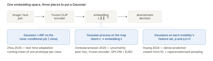
Zhou et al. 2025 — Bayesian Class Adaptation (CVPR) [7]
The observation. CLIP zero-shot classification is usually written as a softmax over cosine similarities. Zhou et al. re-derive it from Bayes’ theorem with M class embeddings \{\mu_m\}:
P(Y \mid x_i) = \sum_{m=1}^{M} P(\mu_m \mid x_i)\, P(Y \mid \mu_m), \qquad P(\mu_m \mid x_i) = \frac{P(x_i\mid\mu_m)P(\mu_m)}{\sum_j P(x_i\mid\mu_j)P(\mu_j)} .
Two factors govern the prediction: the likelihood P(x\mid\mu) and the prior P(Y\mid\mu). Every existing CLIP test-time adaptation method — TPT, DiffTPT, TDA, DOTA — adapts only the likelihood, by moving class embeddings, and leaves the prior at the one-hot value inherited from pre-trained CLIP. Their worked example is good: a patient with a fever is “common cold” under a fixed prior regardless of whether there is a pandemic on. Recovering the standard softmax from their Eq. 4 requires exactly the one-hot prior, which makes the omission visible rather than arguable.
The method. Adapt both, online, without backpropagation. When image x_i arrives: compute its visual embedding; find the most probable class embedding \mu_s; if P(\mu_s\mid x_i) > \tau, update \mu_s by a running mean with the new embedding, and update that class’s prior P(Y\mid\mu_s) by a running mean with the freshly computed posterior. Two counters, two averages, one vector per class. No gradients, constant memory per class.
Where Gaussianity enters. They take P(x_i \mid \mu_m) \propto \exp(\cos(f^v_i, \mu_m)) — a von Mises–Fisher density on the unit sphere — and note explicitly that DOTA instead uses the full Gaussian \mathcal{N}(x\mid\mu_m,\Sigma_m), in which case one would update \Sigma_m as well. The connection to the theory is direct: an isotropic Gaussian conditioned to the unit sphere is a von Mises–Fisher distribution. So the likelihood used here is precisely the spherical shadow of the Gaussian that Betser et al. derive, and the choice between vMF and full Gaussian is the choice between working with normalised or unnormalised features.
The load-bearing consequence is affordance 2 above. A running mean is a principled posterior update only if the class-conditional is an exponential family whose sufficient statistic is the sample mean — a Gaussian with fixed covariance, or a vMF with fixed concentration. If per-class CLIP features were multi-modal or heavy-tailed, one prototype per class would be the wrong summary and averaging would drag it into a low-density region between modes. The paper’s headline selling points — high inference rate, low memory — are not engineering wins that happen to coexist with the Gaussian assumption; they are purchased by it. Drop Gaussianity and you are back to storing a cache of embeddings, which is what TDA does.
Venkataramanan et al. 2025 — GroVE (UAI) [4]
The problem. A frozen VLM gives one point per input, but the image–text relationship is genuinely one-to-many: an image matches many captions and vice versa. Deterministic embeddings cannot express that. Prior probabilistic-embedding work (PCME, PFE, ProbVLM) trains the distributional structure in, which needs large datasets and discards the representations large-scale pre-training already produced.
The method. GroVE is post-hoc on a frozen encoder. Assume each image–text pair’s embeddings z_{I_n}, z_{T_n} \in \mathbb{R}^D are generated from a shared low-dimensional latent x_n \in \mathbb{R}^Q, Q \ll D, by two Gaussian-process mappings:
z_{I_n} = G_I(x_n) + \epsilon_I, \qquad z_{T_n} = G_T(x_n) + \epsilon_T,
with a GP prior per output dimension, g^d \sim \mathcal{N}(m(X), k(X,X)), an RBF kernel, and Gaussian noise \mathcal{N}(g^d, \sigma^2 I). Exact inference is O(N^3), so they use a sparse GP with M inducing points and a Gaussian variational posterior q(u^d) = \mathcal{N}(u^d\mid\mu^d, S^d), trained by maximising the ELBO. A second term aligns the modalities with a symmetric KL between the predicted image and text Gaussians \mathcal{N}(\hat\mu_I,\hat\Sigma_I) and \mathcal{N}(\hat\mu_T,\hat\Sigma_T). At inference, a new embedding z^* has its latent x^* recovered by optimising the ELBO, then pushed through the GP to a predictive Gaussian; the uncertainty score is the mean of \hat\Sigma^*’s diagonal. Retrieval ranks by Wasserstein distance rather than cosine similarity.
Where Gaussianity enters. Everywhere, and more deeply than in the other two. A Gaussian process is a Gaussian assumption on function values, so positing GPs for the map latent \to CLIP-embedding asserts that embedding coordinates are jointly Gaussian given the latent. The noise model is Gaussian, the variational posterior is Gaussian, the predictive distribution is Gaussian, the alignment loss is a Gaussian–Gaussian KL in closed form, and the retrieval metric is a Gaussian Wasserstein distance. Remove the assumption and there is no method left — every one of the four affordances is in use simultaneously.
This makes GroVE the most interesting of the three as evidence. The paper’s headline metric is uncertainty calibration, which is precisely the quantity that degrades when a distributional assumption misfits: a Gaussian noise model over non-Gaussian features would produce confidently wrong variances. They report state-of-the-art calibration across cross-modal retrieval, VQA and active learning on frozen CLIP and BLIP. That is indirect but real empirical support for approximate Gaussianity of the embedding space — arrived at independently of any theory, which is what makes it worth citing in that direction.
C. Huang et al. 2024 — Multimodal Representation Distribution Learning (IJCAI) [8]
The problem. Medical image segmentation is starved of pixel-level labels, so text annotations are used as a cheaper auxiliary signal. But the standard fusions are crude: element-wise addition merges the two feature distributions and keeps everything, including the redundant overlap, while plain contrastive alignment pulls them together without separating what is shared from what is modality-specific.
The method. Introduce K learnable features F_L, initialised near the text prompt feature and perturbed with 0.1\cdot\mathcal{N}(0,I) so they do not collapse to one vector. Then model the text and vision feature distributions in the joint space H as Gaussians, p \sim \mathcal{N}(\mu_p,\sigma_p^2) and q \sim \mathcal{N}(\mu_q,\sigma_q^2), with parameters estimated from \{F_T\}\cup F_L and \{F_V\}\cup F_L respectively. Minimising the closed-form Gaussian KL
\mathcal{L}_{\mathrm{KL}} = \log\frac{\sigma_q}{\sigma_p} + \frac{1}{2\sigma_p^2}\big(\sigma_p^2 + (\mu_p-\mu_q)^2\big) - \frac{1}{2}
drives the learnable features to capture what the modalities share, leaving the residual as modality-specific. The fused feature is then sampled from a learnable Gaussian r = \mathcal{N}(\mu_r,\sigma_r) via the reparameterisation trick F = \mu_r + \omega\sigma_r, so it stays differentiable. A separate frequency prompt encoder takes the FFT phase spectrum — which carries edge and structural information — to supply boundary detail. Training combines Dice, cross-entropy and the KL term.
Where Gaussianity enters. Here it is stated outright as an assumption — “we assume p, q follow Gaussian distributions” — and then everything downstream is a Gaussian formula. This is the clearest instance of the pattern: the assumption is not argued for, it is used, and it buys exactly affordances 1 and 4. The KL expression above is only the divergence between the actual feature distributions if those distributions are in fact Gaussian; otherwise it is a well-defined but differently-meaning penalty on two moments. Likewise the symmetry-breaking noise injection and the sampling of F from r both presume that a feature’s neighbourhood in the joint space is well modelled as a Gaussian ball.
Of the three this is the most casual about the assumption and the most instructive about why the theory is worth having. The method works; the paper offers no account of why a Gaussian is the right object; Betser et al. supply one.
What the theory adds, and where it stops
What it adds. A population-level reason to expect approximate Gaussianity, rather than treating it as a fortunate empirical accident. Concretely: a prediction that the approximation improves with embedding dimension (the Diaconis–Freedman rate is O(1/d), so d = 512 is comfortable and d = 32 is not), and a prediction that it depends on the training objective being contrastive — so the same trick should transfer to SimCLR, MoCo and CLIP, and should be questioned for supervised or reconstruction-trained encoders.
Where it stops, and this matters for all three papers above. Betser et al.’s result is about fixed low-dimensional projections of the representation, and about the marginal distribution. Neither is quite what these methods need:
- Zhou et al. need class-conditional Gaussianity. Betser et al. explicitly disclaim any statement about class structure, and note that well-separated class clusters can coexist with an approximately Gaussian marginal. A Gaussian marginal that is a mixture of well-separated Gaussians is still Gaussian-ish in projection while making a single global prototype per class the right object only if each component is itself unimodal. The theory is consistent with what they need but does not establish it.
- Venkataramanan et al. need joint Gaussianity of many coordinates at once, not of a fixed k-dimensional projection with k small. The spherical CLT’s error grows with k (d_{\mathrm{TV}} \le 2(k+3)/(d-k-3)), so the guarantee weakens exactly in the regime a GP over all D output dimensions occupies.
- C. Huang et al. apply the assumption to features from a medical segmentation encoder trained with Dice and cross-entropy alongside the KL term — not a purely contrastive objective, and not on natural images. Whether the induced-Gaussianity argument transfers is an open question, not a corollary.
So the honest reading is: the theory explains the phenomenon these methods exploit and predicts when it should hold, but each application needs a slightly stronger or differently shaped version of the statement than has been proved. That gap is the interesting place to work.
Questions and doubts
- The evidence is largely indirect. None of these three papers tests Gaussianity of the features they assume Gaussian. Calibration results (GroVE) are suggestive, but a normality diagnostic on the actual embeddings would be a cheap and convincing addition.
- C. Huang et al.’s variance estimator looks wrong as written. Their Eq. 6 defines \sigma_p = \frac{1}{K+1}\big(F_T + \sum_i F^i_L - \mu_p\big)^\top\big(F_T + \sum_i F^i_L - \mu_p\big). But Eq. 5 sets \mu_p = \frac{1}{K+1}(F_T + \sum_i F^i_L), so the bracket equals K\mu_p and the whole expression reduces to \frac{K^2}{K+1}\lVert\mu_p\rVert^2 — a scaled squared norm of the mean, carrying no dispersion information at all. Almost certainly a typo for a sum of per-sample squared deviations. Worth checking against the released code before building on it, since the KL term depends on \sigma.
- Scalar versus full covariance is muddled in the same paper. Eq. 6 is written as an inner product (a scalar) but called a covariance, and the KL of Eq. 10 is the scalar-variance formula. Whether the intended model is isotropic or full-covariance is not resolved in the text.
- Zhou et al.’s prior update has no convergence guarantee. The prior and likelihood are updated from each other’s outputs — the posterior updates the prior, which changes the next posterior. That is a feedback loop, and nothing rules out drift or self-reinforcement of an early mistake. The threshold \tau presumably guards against this but is not analysed.
- Post-hoc methods inherit whatever the frozen encoder did. GroVE’s calibration is evaluated on CLIP and BLIP. If the Gaussian structure is objective-induced, results should differ measurably for an encoder trained non-contrastively — an easy and informative ablation that nobody in this literature seems to have run.
Takeaways
- The applied literature reached “model CLIP features as Gaussian” empirically and independently, across at least five task families. That convergence is itself the strongest evidence that something real is being exploited.
- The assumption is load-bearing in a specific, checkable way: it buys closed-form divergences, sufficiency of mean and covariance, closed-form likelihood, and reparameterised sampling. Naming which affordance a method uses tells you what breaks if the assumption fails.
- The three papers here differ mainly in where they place the Gaussian — on the class-conditional, on the generative map into embedding space, or on each modality’s feature set — and that placement determines what the method can deliver.
- The theory and the applications do not yet meet cleanly. Marginal, low-dimensional-projection Gaussianity is what is proved; class-conditional and high-dimensional joint Gaussianity is what is used.
Sources
The reference list as given in the authors’ rebuttal note zB9oh3CoAg,
preserving its numbering. The three marked ▸ are read in detail
above.
- D. Eftekhari and V. Papyan. On the Importance of Gaussianizing Representations. ICML 2025. Annotated here.
- Anton Baumann et al. Post-hoc Probabilistic Vision–Language Models. arXiv:2412.06014, 2024.
- Pablo Morales-Álvarez et al. BayesAdapter: enhanced uncertainty estimation in CLIP few-shot adaptation. arXiv:2412.09718.
- ▸ Aishwarya Venkataramanan et al. Probabilistic Embeddings for Frozen Vision-Language Models: Uncertainty Quantification with Gaussian Process Latent Variable Models. UAI 2025. arXiv:2505.05163
- Yuning Lu et al. Prompt Distribution Learning. CVPR 2022.
- Zitong Huang et al. Learning Prompt with Distribution-Based Feature Replay for Few-Shot Class-Incremental Learning. arXiv:2401.01598.
- ▸ L. Zhou et al. Bayesian Test-Time Adaptation for Vision-Language Models. CVPR 2025. arXiv:2503.09248
- ▸ C. Huang et al. Multimodal Representation Distribution Learning for Medical Image Segmentation. IJCAI 2024.
- M. Jia et al. Orchestrating the Symphony of Prompt Distribution Learning for Human-Object Interaction Detection. AAAI 2025.
- R. Betser et al. Whitened CLIP as a Likelihood Surrogate of Images and Captions. ICML 2025.
The paper this page hangs off is annotated separately: InfoNCE Induces Gaussian Distribution.