Where is the Information in a Deep Neural Network?
Links
- arXiv:1905.12213: the preprint; these notes follow v5 (22 June 2020). No code is released.
- Interactive companion: four widgets. (1) The Information Lagrangian in one dimension: the exact minimiser, the two Gaussian formulas and the rate–distortion curve. (2) Flat against sharp minima under temperature. (3) The paper’s Figure 3 toy, rerun in the browser, with its Shannon estimate taken apart. (4) Which Fisher the activations see, in a two-weight picture.
- Runnable
checks:
information_checks.pychecks the algebra of Propositions 2.3, 2.5, 2.8, 2.9 and 3.2.hessian_fisher.pychecks Lemma 2.4 on a small network.sgd_toy.pyrebuilds the Figure 3 experiment. Every number below comes from one of them, andmake verifyruns all three. - Inequalities and concentration: the KL chain rule and Donsker–Varadhan sections are the background for Proposition 2.3 and for the Gibbs form of the optimum below.
- Expectation–Maximization: the ELBO, which Definition 2.1 generalises.
- Langevin dynamics: background for Proposition 2.8 and the SGD-temperature picture, built up with simulations: the Gibbs law e^{-U/D}, the free energy of a well (U+\frac D2\log\det H), Eyring–Kramers escape times, and why noise shaped like the Hessian gives a round stationary cloud instead of DH^{-1}.
- Fisher information: background for Sections 2.4–2.5 and 3: the Fisher matrix from the score, its link to the KL divergence and to Cramér–Rao, the three matrices called “Fisher” (model, empirical, Hessian), and why it shares its non-zero eigenvalues with the neural tangent kernel.
- The papers this one builds on: Achille & Soatto, Emergence of invariance and disentanglement in deep representations, JMLR 2018 (arXiv:1706.01350); Hinton & van Camp, Keeping neural networks simple by minimizing the description length of the weights, COLT 1993; McAllester, A PAC-Bayesian tutorial with a dropout bound (arXiv:1307.2118).
Alessandro Achille, Giovanni Paolini and Stefano Soatto, Where is the Information in a Deep Neural Network?, arXiv 2019–2020.
In one paragraph
After training, a network is a fixed function. Its weights are numbers, and the mutual information between a fixed number and anything else is either zero or infinite. So “how much does the network know about its training set?” needs a definition before it has an answer. The paper’s definition is a coding cost. Imagine perturbing the weights with noise Q(w\mid\mathcal D) and measuring (a) how much the training loss rises and (b) how many nats it takes to describe the noisy weights relative to a reference code P(w), which is \mathrm{KL}(Q\,\Vert\,P). The trade-off C_\beta=\mathbb E_Q[L_{\mathcal D}]+\beta\,\mathrm{KL}(Q\Vert P) is the Information Lagrangian, and the KL at its optimum is the Information in the Weights (Definition 2.1). Choosing P and Q recovers the classical quantities. The best P on average over datasets gives Shannon’s mutual information I(w;\mathcal D) (Proposition 2.3), which controls generalisation through PAC-Bayes. Gaussian P and Q give a log-determinant of the Hessian, which is close to the Fisher (Propositions 2.4–2.5). The paper then argues that SGD links the two. Its noise pushes it out of sharp minima (Proposition 2.8, the Eyring–Kramers law), and flatter, more stable minima carry less Shannon information (Proposition 2.9). Finally, weight noise of the size the Fisher allows induces noise in the activations, and that bounds how much information about the input the activations effectively carry (Proposition 3.2). So small information in the weights should force invariant representations. The framework is clean and the definitions are worth knowing. Checking the details, I found three algebra slips, one of them in the central formula of Section 3, plus an approximation used outside the regime where it is valid. The paper’s own toy experiment, rebuilt, does not show what the paper says it shows: the drop in “Shannon information” with small batches is the entropy of which equivalent minimum SGD reaches. That is randomness from the seed, not information about the data.
The spine of the argument
The paper runs a chain of links from quantities you can compute on the training set to properties of the network on unseen data. Here is each link and how it fared under checking:
| Link | Statement | Status after checking |
|---|---|---|
| Def 2.1 | IW = KL at the optimum of \mathbb E_Q L+\beta\,\mathrm{KL}(Q\Vert P) | Clean; the optimum is a Gibbs distribution (§2.1 below) |
| Thm 2.2 | PAC-Bayes: small C_\beta ⇒ small test loss | Standard, but its \beta is N times the \beta of Def 2.1 |
| Prop 2.3 | Optimal P = marginal; \mathbb E\,\mathrm{KL}=I(w;\mathcal D) | Correct; checked exactly |
| Lemma 2.4 | H=F+ residual; H\approx F when points are fitted | Decomposition exact; “residual → 0” true only in absolute terms |
| Prop 2.5 | Gaussian IW ≈ \tfrac12\log\lvert H\rvert + const | Right shape, but \Sigma^* is off by a factor 2 and Eq 8 has -k for -k/2 |
| Prop 2.8 | Higher SGD temperature avoids high-Fisher minima | For equal-loss minima, isotropic Kramers says the preference is independent of T |
| Prop 2.9 | Lower Fisher or more stable SGD ⇒ lower I(w;\mathcal D) | At a minimiser the two are one knob, not two; \beta should be \beta^k |
| Prop 3.2 | Fisher of activations =\frac1\beta\nabla_x f^\top J F_w J^\top\nabla_x f | Should be \nabla_x f^\top(\beta J F_w^{-1}J^\top)^{-1}\nabla_x f; Eq 10 needs \dim z\ge\dim x |
| §3 end | Minimal IW ⇒ invariant activations | Qualitatively plausible; not established by Prop 3.2 |
| §4, Fig 3 | Small batches lower both Fisher and Shannon information | Rebuilt: true Shannon information is flat; the estimator measures the seed |
Background, from the ground up
KL divergence and mutual information, in plain words
\mathrm{KL}(q\Vert p)=\mathbb E_{w\sim q}[\log q(w)/p(w)] is the average number of extra nats you pay when you encode samples of q with a code designed for p. A small example: if q puts all its mass on one of 8 equally likely outcomes of p, then \mathrm{KL}=\log 8, the cost of saying which outcome it was. The same reading works for continuous weights. Take a code P=\mathcal N(0,\lambda^2) for one weight and a “noisy weight” Q=\mathcal N(w^*,\sigma^2). Then \mathrm{KL}(Q\Vert P)=\log(\lambda/\sigma)+\tfrac{\sigma^2+w^{*2}}{2\lambda^2}-\tfrac12. The main term, \log(\lambda/\sigma), is the number of nats needed to pin the weight down to precision \sigma inside a range of size \lambda. A weight that tolerates a lot of noise (large \sigma) is cheap to store.
Mutual information is the same idea averaged over the thing being described: I(w;\mathcal D)= \mathbb E_{\mathcal D}\,\mathrm{KL}(Q(w\mid\mathcal D)\,\Vert\,Q(w)), where Q(w)=\mathbb E_{\mathcal D}Q(w\mid\mathcal D) is the distribution of weights you would get before knowing which dataset you trained on. It asks: how much does seeing the dataset change what the weights look like?
Fisher information: how fast the output distribution moves with the weights
For a model p_w(y\mid x), nudge the weights by \delta w. The output distribution moves, and to second order \mathbb E_x\,\mathrm{KL}(p_w\Vert p_{w+\delta w})=\tfrac12\delta w^\top F\,\delta w with
F=\mathbb E_{x}\,\mathbb E_{y\sim p_w(y\mid x)}\big[\nabla_w\log p_w(y\mid x)\,\nabla_w\log p_w(y\mid x)^\top\big].
(The paper drops the \tfrac12 in Section 1.2; it matters nowhere.) Two things to notice. First, y is drawn from the model, not from the data, so F depends on the inputs x but not on the labels (the paper uses this in Section 2.3). Second, a big F in a direction means a small move there changes the predictions a lot: the weight is “informative” and must be stored precisely. So \tfrac12\log\lvert F\rvert behaves like the \log(1/\sigma) term above, summed over directions.
A one-number example: a single logistic unit with logit z=wx at x=1 has F=p(1-p). That is 0.25 when p=0.5, and \approx 0.0099 when p=0.99. Confident predictions have small Fisher, a fact that returns in the discussion of Lemma 2.4.
PAC-Bayes: generalisation priced in nats
A PAC-Bayes bound says the test loss of a randomised predictor w\sim Q is at most its training loss plus a penalty proportional to \mathrm{KL}(Q\Vert P)/N, for any P fixed before seeing the data. The penalty is the coding cost of the weights, spread over the N training points. If the weights can be described in few nats relative to N, the network cannot have memorised the labels, which would cost about N\log\lvert\mathcal Y\rvert nats. That is the whole motivation for measuring information in the weights by a KL.
Setup and notation
| Symbol | Meaning |
|---|---|
| \mathcal D=\{(x_i,y_i)\}_{i=1}^N | the training set |
| L_{\mathcal D}(w)=\frac1N\sum_i-\log p_w(y_i\mid x_i) | mean cross-entropy on the training set (a mean, not a sum) |
| P(w) | pre-distribution: a reference code chosen before seeing \mathcal D (not a Bayesian prior) |
| Q(w\mid\mathcal D) | post-distribution: a chosen perturbation of the trained weights (not a Bayesian posterior) |
| C_\beta(\mathcal D;P,Q) | Information Lagrangian \mathbb E_Q[L_{\mathcal D}]+\beta\,\mathrm{KL}(Q\Vert P) (Eq 2) |
| H=\nabla^2_w L_{\mathcal D} | Hessian of the training loss |
| F, F_w, F(w) | Fisher information of the weights (labels sampled from the model) |
| k | number of weights (in Prop 2.9’s formula it should be the dimension of \mathcal D) |
| T\propto\eta/B | SGD “temperature”: learning rate over batch size |
| z=f_w(x) | activations of some layer; J_f=\partial z/\partial w, \nabla_x f=\partial z/\partial x |
| I_{\text{eff},\beta}(x;z) | effective information: I(x;z_n) with z_n=f_{w+n}(x), n\sim\mathcal N(0,\beta F^{-1}) |
The paper insists, rightly, that P and Q are choices of code, like choosing a unit of measurement. They are not claims about how SGD distributes the weights. Different choices give different information measures, and the art is to pick the one that connects to what you want to prove.
Section 2: Information in the Weights
2.1 Definition 2.1, and what minimises it
C_\beta(\mathcal D;P,Q)=\mathbb E_{w\sim Q(w\mid\mathcal D)}[L_{\mathcal D}(w)]+\beta\,\mathrm{KL}\big(Q(w\mid\mathcal D)\,\Vert\,P(w)\big).
The first term is the loss the network suffers if its weights are jittered by Q. The second is the cost of describing the jittered weights. A large \beta says “description is expensive”, so Q spreads out and the weights are stored coarsely. A small \beta lets Q shrink onto the minimum.
The paper does not write down the minimiser, but it has a closed form, and it is worth having. Collect both terms under one expectation:
C_\beta=\beta\,\mathbb E_Q\Big[\log Q-\log\big(P\,e^{-L_{\mathcal D}/\beta}\big)\Big] =\beta\,\mathrm{KL}\big(Q\,\Vert\,Q^*_\beta\big)-\beta\log Z_\beta, \qquad Q^*_\beta=\frac{P\,e^{-L_{\mathcal D}/\beta}}{Z_\beta},\quad Z_\beta=\mathbb E_P\,e^{-L_{\mathcal D}/\beta}.
A KL is never negative and is zero only at equality, so the optimal post-distribution is the Gibbs distribution Q^*_\beta\propto P\,e^{-L_{\mathcal D}/\beta}, with optimal value -\beta\log Z_\beta. This is the Donsker–Varadhan identity. Two consequences:
- Differentiating the optimal value in \beta (the envelope theorem: Q^* is optimal, so its own change does not contribute) gives \frac{d}{d\beta}\min_Q C_\beta=\mathrm{KL}(Q^*_\beta\Vert P). The Information in the Weights is the slope of the optimal Lagrangian. As \beta varies, the pairs (\mathrm{KL},\mathbb E L) trace a convex rate–distortion curve, which is the “Pareto-optimal curve” the paper mentions.
- Every Gaussian formula later in the paper is a Laplace approximation of this Gibbs distribution around one minimum.
information_checks.py §2 does this on a grid for a
tilted double well at \beta=0.2. C at the Gibbs distribution is 0.16372, and
200 random perturbations of it are all worse. The best Gaussian is worse
by 0.0786, because it cannot cover both wells. The numerical derivative
of the optimum in \beta is 0.53714, and
so is \mathrm{KL}(Q^*\Vert P).
2.2 Theorem 2.2 (PAC-Bayes), and the two betas
McAllester’s bound, as the paper states it: for a loss in [0,1], any \beta>\tfrac12 fixed in advance, and any Q, with probability at least 1-\delta,
L_{\text{test}}(Q)\le\frac{1}{1-\frac1{2\beta}}\Big[\mathbb E_Q L_{\mathcal D}+\frac{\beta}{N}\big(\mathrm{KL}(Q\Vert P)+\log\tfrac1\delta\big)\Big]. \qquad\text{(Eq 3)}
The bracket has the shape of C_\beta, but with \beta/N where Definition 2.1 has \beta. So the two betas differ by a factor of N: \beta_{\text{Def 2.1}}=\beta_{\text{PAC}}/N. The condition \beta_{\text{PAC}}>\tfrac12 becomes \beta_{\text{Def}}>1/(2N). For N=50\,000 that is \beta>10^{-5}, so “for a sufficiently small \beta” in Proposition 2.5 is compatible with the bound. The same factor of N affects the remark that “\beta=1 coincides with the ELBO”. With L_{\mathcal D} a mean, the negative ELBO divided by N is \mathbb E_Q L_{\mathcal D}+\frac1N\mathrm{KL}, which is \beta=1/N (§4 of the checks prints both values). Two smaller points. The cross-entropy is not bounded by 1, as the theorem needs; footnote 3 defers to McAllester for the reduction. And \beta must be fixed before the data are seen, or paid for with a union bound over a grid.
2.3 Proposition 2.3: Shannon information is the best code on average
Claim. If datasets come from \pi(\mathcal D) and training maps \mathcal D\mapsto Q(w\mid\mathcal D), the P minimising \mathbb E_{\mathcal D}C_\beta is the marginal Q(w)=\mathbb E_{\mathcal D}Q(w\mid\mathcal D), and then \mathbb E_{\mathcal D}\mathrm{KL}(Q\Vert P)=I(w;\mathcal D).
Proof, line by line. Only the KL term involves P. Insert Q(w) inside the log:
\mathbb E_{\mathcal D}\,\mathbb E_{Q(w\mid\mathcal D)}\log\frac{Q(w\mid\mathcal D)}{P(w)} =\mathbb E_{\mathcal D}\,\mathbb E_{Q(w\mid\mathcal D)}\log\frac{Q(w\mid\mathcal D)}{Q(w)} +\mathbb E_{\mathcal D}\,\mathbb E_{Q(w\mid\mathcal D)}\log\frac{Q(w)}{P(w)}.
In the second term, averaging Q(w\mid\mathcal D) over \mathcal D gives Q(w), so it is \mathrm{KL}(Q(w)\Vert P). The first term is I(w;\mathcal D) by definition. Hence \mathbb E_{\mathcal D}\mathrm{KL}(Q\Vert P)=I(w;\mathcal D)+\mathrm{KL}(Q(w)\Vert P)\ge I(w;\mathcal D), with equality exactly at P=Q(w). \square This is the “golden formula” of rate–distortion theory. Checks §1: on a random 5-dataset, 6-weight example both sides are 1.082796, and at P=Q(w) the cost drops to I=0.2994 nats.
Two remarks the paper leaves implicit. The bound needs the algorithm’s Q(w\mid\mathcal D), so any randomness in training (the seed) has to be averaged over, or conditioned on, consistently; Section 4 gets this wrong. And Shannon information is a lower bound on every other choice of P. In particular, no Gaussian code can report fewer nats than I(w;\mathcal D).
2.4 Lemma 2.4: Hessian = Fisher + residual
For logits z=f_w(x) and cross-entropy L(y,z), the chain rule twice gives
H=\frac1N\sum_i J_i^\top\,\nabla_z^2L\,J_i+\frac1N\sum_i\sum_j\big[\nabla_zL(y_i,z_i)\big]_j\,\nabla_w^2 z_{ij}, \qquad J_i=\partial z_i/\partial w.
For softmax cross-entropy, \nabla^2_zL=\operatorname{diag}(p)-pp^\top does not depend on the label. So the first term equals the Fisher (labels drawn from the model) exactly. The second term, the residual, is weighted by \nabla_zL=p-e_{y}. (The paper writes L=-\sum_j\delta_{y,j}\log z_j, which treats z as probabilities. The clean statement is with z as logits.) For a linear model \nabla_w^2z=0 and H=F at every w. The check for logistic regression gives \max\lvert H-F\rvert=1.4\times10^{-12}, which is finite-difference noise.
The paper then says that when “almost all training samples are predicted correctly, \nabla_zL\approx0 and H\approx F”. The first half is true, but it does not give the second. If the correct class has probability 1-\varepsilon, then p-e_y has entries of size \varepsilon. But so does \operatorname{diag}(p)-pp^\top: its (y,y) entry is p_y(1-p_y)\approx\varepsilon. Residual and Fisher shrink together, both O(\varepsilon). So H\approx F holds in absolute terms (both go to zero), but the relative gap is set by the ratio of logit curvature \nabla^2_wz to squared logit gradient \lVert J\rVert^2, an architectural quantity.
hessian_fisher.py measures this on a 2-16-16-1 tanh
network (337 weights) trained by full-batch gradient descent on 200
two-moons points. The Hessian comes from finite differences of the exact
gradient. The decomposition holds at every checkpoint (relative error
below 10^{-8}).
| GD step | train loss | accuracy | \lVert H-F\rVert/\lVert F\rVert | \operatorname{tr}F |
|---|---|---|---|---|
| 30 | 0.30 | 0.87 | 0.41 | 1.36 |
| 100 | 0.107 | 0.975 | 0.17 | 4.56 |
| 300 | 0.0102 | 1 | 0.068 | 2.61 |
| 3 000 | 5\times10^{-4} | 1 | 0.039 | 0.49 |
| 100 000 | 7.7\times10^{-6} | 1 | 0.041 | 0.016 |
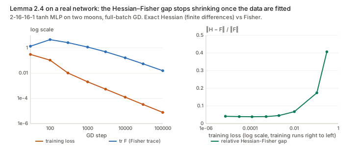
So H\approx F to about 4% here, which is good enough for the paper’s purposes. But the gap stops improving once the data are fitted: from step 3 000 on, the loss falls another factor of 70 and the gap does not move. Two side observations matter for Figures 1 and 4. First, the Fisher trace peaks at step 100 and then falls 293-fold while the decision boundary barely changes. Once points are classified confidently, p(1-p)\to0. A late “compression” of the Fisher on separable data therefore needs no change in what the network computes, only more confident logits. Second, at a fitted minimum the Hessian has tiny negative eigenvalues (the most negative is -4\times10^{-6}), which is why Remark 2.6 prefers the Fisher, which is positive semi-definite by construction.
2.5 Proposition 2.5: the Gaussian (Fisher) Information in the Weights
Setting. P=\mathcal N(0,\lambda^2I) and Q=\mathcal N(w^*,\Sigma) centred at a local minimum w^*. Find the best \Sigma and the resulting KL.
Derivation, with the step the paper slips on. For small \beta, Q is concentrated near w^*, where L_{\mathcal D}(w)\approx L_{\mathcal D}(w^*)+\tfrac12(w-w^*)^\top H(w-w^*) (the gradient vanishes at a minimum). The expected loss under Q is then
\mathbb E_Q L_{\mathcal D}=L_{\mathcal D}(w^*)+\tfrac12\operatorname{tr}(H\Sigma),
because \mathbb E[(w-w^*)^\top H(w-w^*)]=\operatorname{tr}(H\,\mathbb E[(w-w^*)(w-w^*)^\top])=\operatorname{tr}(H\Sigma). The Gaussian KL is
\mathrm{KL}(Q\Vert P)=\tfrac12\Big[\tfrac{\operatorname{tr}\Sigma+\lVert w^*\rVert^2}{\lambda^2}-k+k\log\lambda^2-\log\lvert\Sigma\rvert\Big].
Setting \partial C_\beta/\partial\Sigma=\tfrac12H+\tfrac{\beta}{2\lambda^2}I-\tfrac\beta2\Sigma^{-1}=0 gives
\boxed{\Sigma^*=\beta\Big(H+\frac{\beta}{\lambda^2}I\Big)^{-1}}\qquad\text{(paper: }\Sigma^*=\tfrac\beta2\big(H+\tfrac{\beta}{2\lambda^2}I\big)^{-1}\text{)}.
The appendix proof writes \mathbb E_QL_{\mathcal D}\simeq L_{\mathcal D}(w^*)+\operatorname{tr}(H\Sigma), without the \tfrac12 of the Taylor expansion. The paper’s \Sigma^* is exactly the optimum of that objective (checks §3: the paper’s objective has gradient 1.6\times10^{-15} at the paper’s \Sigma^*). Against the correct objective, the gradient there is 1.6, while at \beta(H+\beta/\lambda^2I)^{-1} it is 4\times10^{-16}. There is an independent check. For a quadratic loss, the exact Gibbs minimiser from §2.1 is Gaussian with covariance (H/\beta+I/\lambda^2)^{-1}, which is the corrected formula. So the paper’s perturbation is half as wide as it should be: the ratio of traces is 0.506 at \beta=0.01, tending to \tfrac12. The cost of using it is \beta(\tfrac12\ln2-\tfrac14)\approx0.097\beta nats per weight of extra Lagrangian (0.572\beta for the 6-weight example). The paper’s own later sections quietly use the corrected size: Definition 3.1 and Proposition 2.9 both take \beta F^{-1}, which is the \lambda\to\infty limit of the corrected \Sigma^*, not of the stated one.
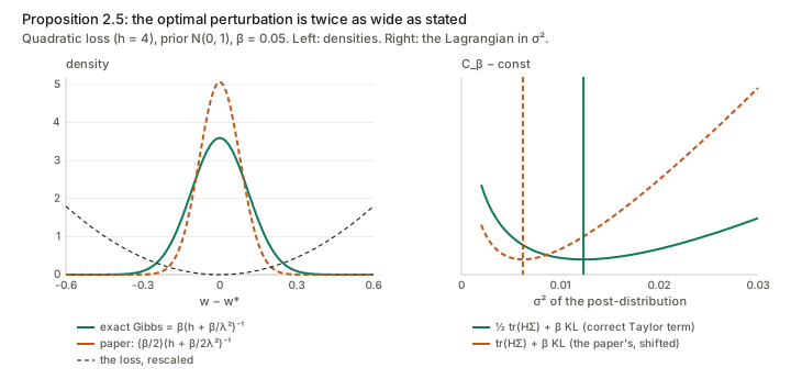
Substituting the corrected \Sigma^* (using \log\lvert\Sigma^*\rvert=k\log\beta-\log\lvert H+\tfrac\beta{\lambda^2}I\rvert):
\mathrm{KL}(Q^*\Vert P)=\tfrac12\log\Big\lvert H+\tfrac{\beta}{\lambda^2}I\Big\rvert+\tfrac k2\log\tfrac{\lambda^2}{\beta}-\tfrac k2 +\tfrac1{2\lambda^2}\Big[\lVert w^*\rVert^2+\beta\operatorname{tr}\big(H+\tfrac\beta{\lambda^2}I\big)^{-1}\Big].
Eq (8) in the paper has the same structure with its own \Sigma^*, but ends the first line with -k. Evaluating the KL at the paper’s own \Sigma^* gives -k/2. The check finds Eq (8) as printed is 12.8454 and the true KL is 15.8454, a difference of exactly k/2=3. None of this changes the paper’s qualitative message, because the dependence on the minimum is carried by \tfrac12\log\lvert H\rvert in both versions. The slips shift additive constants.
How to read the formula: for small \beta each eigen-direction of H with eigenvalue h_i\gg\beta/\lambda^2 contributes \tfrac12\log(h_i\lambda^2/\beta) nats. That is “the weight must be stored to precision \sqrt{\beta/h_i} in a range of size \lambda”. Flat directions (h_i\lesssim\beta/\lambda^2) cost nothing. Remark 2.7 is right that the \lambda\to\infty limit leaves \tfrac12\log\lvert H\rvert plus a diverging constant.
2.6 Proposition 2.8: Eyring–Kramers and the free energy
The law. For overdamped Langevin dynamics dw=-\nabla L\,dt+\sqrt{2T}\,dW, the expected time to leave a minimum w^* over a saddle w^s with one negative eigenvalue \lambda_1(w^s) is, as T\to0,
\mathbb E\tau=\frac{2\pi}{\lvert\lambda_1(w^s)\rvert}\sqrt{\frac{\lvert\det H(w^s)\rvert}{\det H(w^*)}}\;e^{(L(w^s)-L(w^*))/T}.
Where the free energy comes from. Write the square root as an exponential: \sqrt{\lvert H_s\rvert/\lvert H_*\rvert}=\exp\big(\tfrac1T[\tfrac T2\log\lvert H_s\rvert-\tfrac T2\log\lvert H_*\rvert]\big). Then \mathbb E\tau=\frac{2\pi}{\lvert\lambda_1\rvert}e^{(\mathcal F(w^s)-\mathcal F(w^*))/T} with \mathcal F=L+\tfrac T2\log\lvert H\rvert. That is the paper’s formula, with H replaced by the Fisher. (At a saddle the Hessian has a negative eigenvalue and the Fisher does not, so that substitution needs more care there than at a minimum.) The same \mathcal F is also the Laplace approximation to the Gibbs mass of a basin: \int_{\text{basin}}e^{-L/T}\approx e^{-L(w^*)/T}(2\pi T)^{k/2}\lvert H_*\rvert^{-1/2}\propto e^{-\mathcal F(w^*)/T}.
The catch. The T in front of \log\lvert H\rvert is divided out again in the exponent. The curvature enters \mathbb E\tau only through the T-independent prefactor \lvert H_*\rvert^{-1/2}. Take two minima with the same loss, which is the normal situation for an overparameterised network at zero training loss. Then the ratio of their escape times, and the ratio of their Gibbs masses, is \sqrt{\lvert H_B\rvert/\lvert H_A\rvert} at every temperature. The flat minimum is preferred, but raising T does not make it more preferred. Temperature only trades loss against volume: it matters when the flat minimum is also higher.
Checks §5, with exact 1-D mean first-passage times (no Kramers approximation) for a well of curvature 100 and one of curvature 1 at equal depth:
| T | \mathbb E\tau sharp / \mathbb E\tau flat | Gibbs share of the sharp well | same, flat well 0.25 higher |
|---|---|---|---|
| 0.1 | 0.1007 | 0.0930 | 0.213 |
| 0.2 | 0.0951 | 0.0955 | 0.138 |
| 0.3 | 0.0890 | 0.0985 | 0.122 |
The Laplace prediction for the equal-depth share is 0.1/1.1=0.0909 at every T. The small drift at higher T goes towards the sharp well, the opposite of the claim. Only when the flat well is lifted does higher T push mass into it.
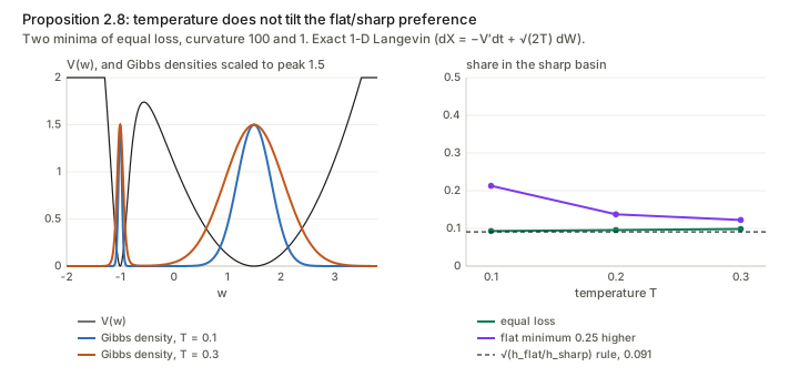
So the isotropic law, which is what Proposition 2.8 states, does not support “increasing the temperature makes the optimisation more likely to avoid minima with high Fisher” for degenerate minima. The paper says the anisotropic case shares the tendency. It does, but for a different reason. SGD’s noise covariance is itself roughly proportional to the Hessian near a minimum, so a sharp minimum is also a hot one, and the curvature moves into the exponent (Xie et al. 2020). The toy in Section 4 shows exactly this. Started from its own stationary distribution, isotropic Langevin keeps the distribution over equal-loss minima where it is at every temperature, and only SGD noise moves it.
2.7 Proposition 2.9: Shannon ≈ Fisher, via Brunel–Nadal
The tool. Brunel & Nadal (1998): if a parameter \theta\in\mathbb R^d is observed through data r precise enough that the posterior p(\theta\mid r) is nearly Gaussian with covariance J(\theta)^{-1} (the inverse Fisher of r about \theta), then its conditional entropy is about \mathbb E\,\tfrac12\log\big((2\pi e)^d/\lvert J\rvert\big). So I(\theta;r)\approx H(\theta)-\mathbb E\,\tfrac12\log\big((2\pi e)^d/\lvert J(\theta)\rvert\big). Plainly: the information equals the prior uncertainty minus the uncertainty that remains, and the remainder is the volume of the Fisher ellipse.
Application. The “parameter” is the dataset \mathcal D (parameterised by d numbers) and the “observation” is w\sim\mathcal N(w^*(\mathcal D),\beta F^{-1}). For a Gaussian whose mean moves with \mathcal D, the Fisher about \mathcal D is \nabla_{\mathcal D}w^{*\top}(\beta F^{-1})^{-1}\nabla_{\mathcal D}w^*=\tfrac1\beta\nabla_{\mathcal D}w^{*\top}F\,\nabla_{\mathcal D}w^* (the covariance-derivative term is dropped by the footnote-5 assumption). Its determinant is \beta^{-d}\lvert\nabla w^{*\top}F\nabla w^*\rvert, so
I(w;\mathcal D)\approx H(\mathcal D)-\mathbb E_{\mathcal D}\Big[\tfrac12\log\frac{(2\pi e\,\beta)^d}{\lvert\nabla_{\mathcal D}w^{*\top}F(w^*)\,\nabla_{\mathcal D}w^*\rvert}\Big].
The paper has \beta(2\pi e)^k: \beta should be raised to the power d, and d is the dimension of \mathcal D (the Brunel–Nadal parameter), not the number of weights. Another constant shift.
The interpretation needs a correction. The paper reads this as two independent levers: “reducing the Fisher (flatness), or making SGD more stable, i.e. reducing \nabla_{\mathcal D}w^*, both reduce I(w;\mathcal D).” At an actual minimiser the levers are welded together. Differentiate the stationarity condition \nabla_wL(w^*(\mathcal D);\mathcal D)=0 in \mathcal D: H\,\nabla_{\mathcal D}w^*+\partial_{\mathcal D}\nabla_wL=0, so \nabla_{\mathcal D}w^*=-H^{-1}\partial_{\mathcal D}\nabla_wL. A flatter minimum (smaller H) moves more when the data change. With F\approx H,
\nabla_{\mathcal D}w^{*\top}F\,\nabla_{\mathcal D}w^*\approx\partial_{\mathcal D}\nabla_wL^\top\,H^{-1}\,\partial_{\mathcal D}\nabla_wL,
so at fixed data-sensitivity of the gradient, flatness raises the information. More basically, the whole expression is invariant under reparameterising the weights, as mutual information must be. Checks §6 does least squares with the labels as the dataset coordinates. There \tfrac1\beta J^\top HJ is exactly \tfrac2{N\beta} times the hat matrix X(X^\top X)^{-1}X^\top (max deviation 8\times10^{-17}). A reparameterisation that makes the minimum 100 times flatter (Hessian trace 10.634 → 0.1063) makes it 10 times less stable (\lVert\nabla_yw^*\rVert 0.371 → 3.715) and leaves the product unchanged (6\times10^{-17}). This is the information-theoretic face of Dinh et al.’s observation that sharpness is not reparameterisation invariant, which the paper cites. What is meaningful is the combination the formula actually contains: how far the minimum moves when the data change, measured in the metric F/\beta. That is precisely the ellipse comparison in Figure 2, so the figure is on firmer ground than the sentence beside it.
Also note: the rank of \tfrac1\beta J^\top HJ is at most the number of weights. With d=40 label coordinates and 5 weights it has rank 5, the determinant is zero, and the formula returns -\infty. So Brunel–Nadal needs \dim\mathcal D\le\dim w: an overparameterised model and a low-dimensional parameterisation of datasets.
Section 3: effective information in the activations
3.1 Definition 3.1
The activations z=f_w(x) are a deterministic function of x, so I(x;z) is degenerate. The paper borrows the noise from the weights. Perturb w by n\sim\mathcal N(0,\beta F^{-1}), the largest perturbation the Lagrangian tolerates, and call I_{\text{eff},\beta}(x;z)=I(x;f_{w+n}(x)) the effective information. The idea is attractive: input features that survive only in directions the weights “do not care about” are washed out by this noise, so the effective information counts only what the trained classifier actually uses.
3.2 Proposition 3.2 (i): which Fisher do the activations carry?
Derivation. Linearise in the weights: z_n=f_{w+n}(x)\approx f_w(x)+J_f\,n. Given x, z_n is therefore Gaussian,
z_n\mid x\;\sim\;\mathcal N\big(f_w(x),\;\Sigma(x)\big),\qquad \Sigma(x)=J_f\,(\beta F_w^{-1})\,J_f^\top.
This is a pushforward: the weight-noise covariance \beta F_w^{-1} is carried into activation space by J_f. The Fisher of a Gaussian family \mathcal N(m(x),\Sigma(x)) about x has a mean part and a covariance part:
[F_{z\mid x}]_{ab}=\partial_a m^\top\Sigma^{-1}\partial_b m+\tfrac12\operatorname{tr}\big(\Sigma^{-1}\partial_a\Sigma\,\Sigma^{-1}\partial_b\Sigma\big).
The covariance part does not depend on \beta (the \beta’s cancel), while the mean part is O(1/\beta). So for small \beta the mean part dominates:
\boxed{F_{z\mid x}\approx\nabla_xf^\top\big(\beta\,J_fF_w^{-1}J_f^\top\big)^{-1}\nabla_xf} \qquad\text{(paper: }\tfrac1\beta\nabla_xf^\top J_fF_wJ_f^\top\nabla_xf\text{)}.
The paper’s version puts F_w where (J_fF_w^{-1}J_f^\top)^{-1} belongs. In the appendix the last line reads \nabla_xf\cdot\Sigma_w^{-1}\nabla_xf, applying the weight-space precision directly to activation-space vectors, and the main text then sandwiches it between J_f’s. A dimensional check shows the problem. If w has units [w] and z units [z], then F_w\sim[w]^{-2} and J_f\sim[z]/[w]. So J_fF_w^{-1}J_f^\top\sim[z]^2 is a covariance, and its inverse is a precision. But J_fF_wJ_f^\top\sim[z]^2/[w]^4 is neither.
Checks §7 uses a linear layer z=Wx with a K-FAC-shaped Fisher F_w=A\otimes B, \dim z=3, \dim x=5. The exact Gaussian Fisher agrees with a Monte Carlo estimate of \mathbb E[-\nabla_x^2\log p(z\mid x)] to 0.5%. The mean term has trace 111.0, the covariance term 4.3, and the paper’s formula gives 386.0. For this Kronecker case the ratio of the paper’s formula to the correct one is exactly (x^\top Ax)(x^\top A^{-1}x). For unit x, Kantorovich’s inequality puts that ratio in [1,(\kappa+1)^2/4\kappa]. So the paper overstates the Fisher, here by 3.48 (1.37 after normalising x). It also gets the dependence on the input scale backwards. Doubling x multiplies the correct Fisher by 0.25, because weight noise acting on a larger input makes larger activation noise. The paper’s formula instead multiplies it by 4.
The discrepancy is largest when weights are correlated. One activation z=w_1x reads one of two weights whose Fisher is \left(\begin{smallmatrix}1&\rho\\\rho&1\end{smallmatrix}\right):
| \rho | correct (JF^{-1}J^\top)^{-1} | paper JFJ^\top |
|---|---|---|
| 0 | 1.000 | 1.000 |
| 0.9 | 0.190 | 1.000 |
| 0.99 | 0.020 | 1.000 |
With \rho near 1 the two weights are nearly redundant. Noise can move w_1 freely as long as w_2 compensates, so w_1 is barely constrained, and the correct formula (a Schur complement, 1-\rho^2) sees that. The paper’s formula looks only at the diagonal entry and misses it. Widget 4 of the interactive page draws this.
What survives: both expressions scale like c when F_w\to cF_w, and both are monotone in F_w in the matrix order (F\preceq F' implies F^{-1}\succeq F'^{-1}, and so on through the inverse). So the qualitative claim (i), “the Fisher of the activations goes to zero when the Fisher of the weights goes to zero”, holds for the corrected formula too. So does “a smaller Lipschitz constant \nabla_xf reduces it”. (The statement also defines F_{z\mid x}=\mathbb E[\nabla_x^2\log p] without the minus sign; the proof has it.)
3.3 Proposition 3.2 (ii): the dimension problem in Eq (10)
Eq (10) applies Brunel–Nadal again, now with x as the parameter: I_{\text{eff}}(x;z)\approx H(x)-\mathbb E\,\tfrac12\log\big((2\pi e)^{\dim x}/\lvert F_{z\mid x}\rvert\big). But F_{z\mid x} is a \dim x\times\dim x matrix built from \nabla_xf, which has only \dim z rows. Its mean part has rank at most \dim z. For any layer narrower than the input, say 10 logits for a 3 072-pixel image, the determinant is zero and the formula returns -\infty. In the check, the mean term has rank 3, the covariance term rank 1, and the sum rank 4 < 5: the smallest eigenvalue is 5.5\times10^{-15}. The proposition does state the needed assumption: “if p(x\mid z) concentrates around its maximum”. But that assumption says the representation determines the input up to small noise, which is the opposite of the invariant, compressed representations the section is trying to explain. For the representations of interest the approximation is simply unavailable. What remains valid is part (i) and the qualitative “less weight Fisher, less input sensitivity” message.
3.4 From effective information to invariance
The section closes by combining (i) with Proposition 3.1 of Achille & Soatto (2018). There, a sufficient representation is maximally invariant to all nuisances if and only if I(x;z) is minimal among sufficient representations. The conclusion is “a network with minimal information in the weights is forced to learn a representation that is effectively invariant to nuisances”. Two gaps. First, nothing shows that the noisy activations z_n remain sufficient for the task, which the cited equivalence requires. Second, (ii) is not available for compressive layers. So the chain low IW → low weight Fisher → low activation Fisher is sound (with the corrected formula). The final step → minimal effective information among sufficient representations → invariance is an interpretation, not a proof.
Section 4: the experiments
4.1 Figure 3, rebuilt: what small batches actually change
The paper’s toy. Draw \mu\sim\mathrm{Unif}[-1,1] and a dataset of N=100 points x_i\sim\mathcal N(\mu,1). Fit \mu by minimising L_{\mathcal D}(\theta)=\frac1N\sum_i(x_i-\varphi(\theta))^2, where \varphi is a fixed zigzag that is steep near \theta=0 and shallow far away (Figure 3, right). Every linear piece of the zigzag sweeps the whole range [-1,1], so every piece holds exactly one global minimum, all with the same loss. They differ only in slope s, hence in curvature 2s^2 and Fisher Ns^2. The paper runs SGD with several batch sizes. It takes Q(\theta\mid\mathcal D)=\mathcal N(\theta^*,F^{-1}) for the minimum \theta^* that each run reaches, and it reports \mathbb E_{\mathcal D}\mathrm{KL}(Q(\theta\mid\mathcal D)\Vert Q(\theta)) as “Shannon information”. Smaller batches give lower Fisher and lower information (3.8 → 2.4 nats).
The rebuild (sgd_toy.py; unstated choices are
mine and are listed in the script). There are 10 pieces on each side,
widths growing by 1.4, slopes 93 to 4.5. \mu\sim\mathrm{Unif}[-0.8,0.8], so that the
minimum sits inside a piece. The learning rate is 10^{-4}, just stable in the steepest piece.
Runs last 20 000 steps, with 300 datasets × 12 runs, and minibatch noise
of the exact variance of sampling B of
N. \theta_0\sim\mathrm{Unif}[-0.5,0.5], because
the paper’s GD histogram sits inside \lvert\theta\rvert<0.7. Three estimates of
information are compared:
- paper’s estimator: one Gaussian per run, averaged KL to the pooled mixture;
- I(\theta;\mathcal D): the same, but the runs of each dataset are averaged into Q(\theta\mid\mathcal D) first. This is the quantity Proposition 2.3 and PAC-Bayes are about;
- H(\text{piece}): the entropy of which zigzag piece the run ends in.
| \mathbb E\log F | H(\text{piece}) | paper’s estimator | I(\theta;\mathcal D) | best Gaussian IW | |
|---|---|---|---|---|---|
| B=100 (GD) | 10.84 | 2.45 | 3.95 | 1.54 | 4.18 |
| B=16 | 10.77 | 2.39 | 3.85 | 1.56 | 4.15 |
| B=4 | 10.64 | 2.32 | 3.70 | 1.59 | 4.10 |
| B=1 | 10.36 | 2.19 | 3.42 | 1.61 | 4.03 |
| Langevin T=0.01 | 10.82 | 2.48 | 3.95 | 1.56 | 4.18 |
| Langevin T=0.16 | 10.65 | 2.57 | 3.98 | 1.56 | 4.18 |
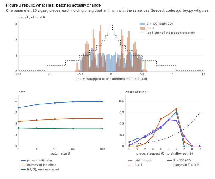
The qualitative trend of the paper’s Figure 3 is reproduced: smaller batches empty the steep central pieces, and both the mean log Fisher and the paper’s estimator fall (3.95 → 3.42). But the estimator is not measuring information about the data.
- Every piece carries the same information about the data. Push a piece’s Gaussian \mathcal N(\theta^*,1/(Ns^2)) through \varphi and it becomes \mathcal N(\bar x,1/N), whatever the slope. That is the reparameterisation invariance of §2.7 in its simplest form. The information inside one piece works out to 1.51 nats (computed directly), and for GD the paper’s estimator minus H(\text{piece}) is exactly 1.51.
- The paper’s estimator is I(\theta;\mathcal D,\text{seed}). One Gaussian per run conditions on the initialisation and the SGD noise, and the pooled mixture averages over them. The excess over I(\theta;\mathcal D) is H(\text{piece}\mid\mathcal D): randomness about which equivalent minimum was reached. For GD that is 3.95 − 1.54 = 2.41 nats, against H(\text{piece})=2.45. For B=1 it is 3.42 − 1.61 = 1.81. So the whole 0.53-nat drop that the paper attributes to less information is this seed entropy falling by 0.60 nats.
- The true I(\theta;\mathcal D) does not fall with batch size. It goes 1.54 → 1.61, a slight rise, because with small batches the piece a run escapes to starts to depend on \bar x (the barriers at the two ends of a piece are (1\mp\bar x)^2). Meanwhile \mathbb E\log F falls by 0.48. In this toy, lower Fisher and lower Shannon information are not linked at all.
- Isotropic Langevin behaves differently from SGD. Its stationary distribution puts mass on each piece in proportion to the piece’s width at every temperature, which is the T-independence of §2.6. Start it from a uniform initialisation over [-1.5,1.5], which already puts runs in proportion to width, and the shares stay put for T=0.01 to 0.16 (the paper’s estimator reads 4.12 to 4.09). From the centred start, higher T only mixes runs towards that width-proportional spread. H(\text{piece}) rises (2.48 → 2.57) and the estimator does not fall (3.95 → 3.98). Only SGD, whose noise in \theta scales with the slope, empties the steep pieces below their width share. From the uniform start its effect shrinks to 0.21 nats, and I(\theta;\mathcal D) sits at 1.55–1.56 throughout.
- “4000–5000 nats” cannot be right for this one-parameter model. The best proper Gaussian code gives 4.0–4.4 nats here. It can never be below the Shannon value (Proposition 2.3), and for a scalar weight it is about \tfrac12\mathbb E\log(\lambda^2F). Reaching thousands of nats would take F\sim e^{8000}. My guess is that the number is the Fisher itself: the Fisher axis of the paper’s Figure 3 is labelled ×10⁴ and peaks near 8 000.
Widget 3 of the interactive page reruns this in the browser.
4.2 Figures 1, 2 and 4
- Figure 1 plots \log\lvert F\rvert (about 0 to 450) over training a 3-layer network on 2-D points, with “bumps” as features are learned and a “compression” at the end. The details are referenced as “see ??”, a broken cross-reference. With more weights than training points the Fisher of a binary classifier is singular, so some damping must have been used, and its size sets the scale of the plot. The late compression has the mundane explanation measured in §2.4: once points are confidently classified, p(1-p) collapses, and the Fisher trace falls 293-fold with no change in the decision boundary.
- Figure 2 shows two SGD paths on datasets differing in one example, against the inverse-Fisher ellipse. As §2.7 argues, the distance between endpoints measured in that ellipse’s metric is the meaningful, invariant quantity. The figure is a single pair of runs, so it illustrates rather than tests.
- Figure 4, left: the Fisher trace after 30 epochs of a ResNet-18 on CIFAR-10 falls with smaller batches. This is consistent with Proposition 2.8 in its anisotropic form. At a fixed number of epochs, smaller batches also mean more steps, and the effect is also predicted by the edge-of-stability picture of the learning rate (sharpness \approx2/\eta), so it does not single out the mechanism.
- Figure 4, right: training on the first k classes gives a smaller final Fisher trace. The paper reads this as “less information in the dataset”. But fewer classes also means fewer training points (5 000 per class), and probably fewer output units. For a fitted softmax the Fisher is a sum over outputs of p_j(1-p_j)-weighted terms, so it grows with k on its own. The experiment does not separate these.
Questions and doubts
- Is the Information in the Weights a property of the network, or of the code? It depends on P, Q and \beta, and the paper embraces this. But then “SGD reduces the information in the weights” is only meaningful for a fixed code, and the two codes the paper uses (Shannon’s and the Gaussian) respond differently to the same change. The toy shows it: mean log Fisher falls 0.48 while I(\theta;\mathcal D) rises 0.07.
- Should the Gaussian IW be reparameterisation invariant? \tfrac12\log\lvert F\rvert is not: rescaling a layer changes it by k\log c. Shannon’s I(w;\mathcal D) is invariant. So the approximate identity of Proposition 2.9 cannot hold as “Fisher equals Shannon”. It holds only as “the invariant combination \nabla w^{*\top}F\nabla w^* equals Shannon”, and that combination is not the one SGD is said to minimise.
- Where does SGD’s flat-minimum bias actually come from? In the isotropic law, temperature does not change the preference among equal-loss minima (§2.6). In the toy, only slope-proportional noise moved runs. So the right citation for the paper’s mechanism is the anisotropic analysis, and the free energy L+\tfrac T2\log\lvert F\rvert is not the thing that explains it. Is there a clean statement of how SGD’s stationary or finite-time distribution over equal-loss minima depends on \eta/B?
- How much of Section 3 survives the corrected Fisher? Claim (i)’s monotonicity does. The formula’s input-scale dependence flips and the correlated-weight case changes by orders of magnitude, so any quantitative use (for example, estimating effective information from a diagonal Fisher) would need the Schur-complement form (J F^{-1}J^\top)^{-1}, not JFJ^\top. With a diagonal Fisher the two coincide only when J reads a single weight per activation.
- What is a usable notion of effective information for compressive layers? Eq (10) is -\infty whenever \dim z<\dim x. One could apply Brunel–Nadal to a low-dimensional parameterisation of the nuisance instead of the whole input, which is what the invariance argument needs anyway. The paper does not do this.
- Does the PAC-Bayes route produce anything non-vacuous here? The paper itself says the Gaussian IW of a DNN is far larger than N\log\lvert\mathcal Y\rvert. So Theorem 2.2 is used for its form, not its values, and the generalisation claims are only as strong as the unproved link between the Fisher and Shannon versions.
- Is the “compression phase” in Figure 1 anything more than logit saturation? Measuring a temperature-scaled or calibrated Fisher (with the logit scale divided out) would separate “the network forgot something” from “the network became more confident”.
- Minor slips, for the record: \Sigma^* off by 2 and -k for -k/2 in Eq 8 (§2.5); the ELBO is \beta=1/N (§2.2); \beta should be \beta^d with d=\dim\mathcal D in Proposition 2.9; the Prop 3.2 statement omits a minus sign; the final formula of the Prop 3.2 proof has T where \beta is meant; “see ??” in Section 2.2; and a paragraph of the Discussion is printed twice.
Takeaways
- The definition is the contribution. Information in a trained network is only defined relative to a code. \min_Q\mathbb E_QL+\beta\,\mathrm{KL}(Q\Vert P) is a natural code, its optimum is the Gibbs distribution P\,e^{-L/\beta}, and the Information in the Weights is the slope of the optimum in \beta. Shannon (averaged P) and Fisher (Gaussian P, Q) are special cases.
- The Gaussian IW is \tfrac12\log\lvert H\rvert plus constants, with the optimal perturbation \beta(H+\beta/\lambda^2)^{-1}, which is twice the paper’s.
- Flatness and stability are one invariant quantity, \nabla_{\mathcal D}w^{*\top}F\,\nabla_{\mathcal D}w^*, which is how far the minimum moves when the data change, in the Fisher metric. Neither sharpness nor sensitivity alone carries information.
- Temperature does not penalise curvature among equal-loss minima under isotropic noise. SGD’s bias comes from its noise scaling with curvature.
- Weight noise reaches the activations through a pushforward, J\,\beta F^{-1}J^\top, whose inverse is the activation precision. Small weight Fisher means noisy activations and less input sensitivity, which is the robust core of Section 3.
- Measure Shannon information with the seed averaged out. Otherwise a redundant parameterisation reports the entropy of which equivalent minimum was reached as if it were information about the data.