Amari's Information Geometry, Chapter 1: manifolds, divergences and the dually flat structure
Links
- Interactive companion: three widgets on the three-outcome probability triangle. (1) Drag two distributions and watch the e-geodesic (straight in the logits), the m-geodesic (straight in the probabilities) and the Fisher–Rao geodesic part ways. (2) Build a right-angled triangle and tilt it away from the right angle to see the Pythagorean theorem fail by exactly the amount the proof predicts. (3) Project a point onto a straight line or a curved arc, for either order of the KL divergence, and count the critical points.
- Runnable
checks:
code/dually_flat.pyprints every number on this page and regenerates the figures withpython3 code/dually_flat.py --figures.make verifyruns it, in about a second. - The book: Amari, Information Geometry and Its Applications (Springer, 2016), DOI 10.1007/978-4-431-55978-8. These notes cover Chapter 1 only. Equation numbers such as (1.69) refer to the book. No text of the book is reproduced here; everything is restated and re-derived.
- Background pages this one leans on: The Fisher information matrix (the metric g of §2 is the Fisher matrix when the family is a statistical model; natural gradient is §7 there), EM and Gaussian mixtures (the alternating projections of §6 are the geometric reading of EM).
- Papers in this collection that use this geometry: Gao & Chaudhari 2021 and Karczewski et al. 2026.
In one paragraph
Take a family of probability distributions, say the outputs of a 3-class softmax classifier. Two coordinate systems describe it equally well: the logits \theta and the probabilities \eta. Neither is “right”, but each makes a different kind of path look straight. The chapter’s idea is that one convex function \psi builds a whole geometry. Its gap above its own tangent is a divergence D_\psi (an asymmetric stand-in for squared distance); its slope \eta=\nabla\psi(\theta) is the second coordinate system (the Legendre transform); and its curvature G=\nabla^2\psi is a metric that turns the divergence into a local squared length. For softmax, \psi is log-sum-exp, \eta is the softmax output, \psi^* is the negative entropy and D_\psi is the KL divergence with its arguments reversed. The payoff is a Pythagorean theorem: if the \eta-straight line from P to Q meets a \theta-straight line from Q to R at a right angle (in the metric G), then D(R{:}P)=D(Q{:}P)+D(R{:}Q) exactly, not just approximately. From it follow the projection theorem (the closest point on a flat family is where the orthogonality holds, and it is unique), and the alternating minimisation that underlies EM and iterative scaling. Almost everything in the rest of the book is this chapter applied to something.
The spine of the argument
- A manifold is a space where each point can be labelled by n numbers; relabelling is allowed. Probability families, positive measures, positive-definite matrices and weight spaces all qualify (§1).
- A divergence D[P{:}Q] is a non-negative, zero-only-at-equality function that looks like a positive-definite quadratic form for nearby points. That quadratic form is a Riemannian metric g, so a divergence gives a manifold a geometry for free (§2).
- Convexity gives divergences on demand: gap of a convex function above its tangent plane = Bregman divergence, and its metric is the Hessian (§3). Exponential families are the example that matters: \psi is their normaliser, \nabla\psi the mean, \nabla^2\psi the covariance, and D_\psi a KL divergence.
- Slopes are coordinates too. The Legendre transform \eta=\nabla\psi(\theta) is invertible, its potential \psi^* is convex, G^*=G^{-1}, and the divergence of the dual is the divergence of the primal with the two arguments swapped (§4).
- So the manifold carries two flat structures at once, one straight in \theta, one straight in \eta, joined by one metric. Vectors have two sets of components that pair up without needing the metric (§5).
- A right angle between a straight line of one kind and a straight line of the other kind makes D additive: Pythagoras. Everything else, projections, uniqueness, alternating minimisation, is a corollary (§6).
Setup and notation
The running example throughout is a 3-class softmax, because it makes every object concrete.
| Chapter-1 object | In the softmax example | Name in the book |
|---|---|---|
| point P | a distribution p=(p_0,p_1,p_2) | point of a manifold |
| \theta | logits relative to class 0: \theta_i=\log(p_i/p_0), i=1,2 | affine coordinates; “natural parameters” |
| \eta=\theta^* | probabilities (p_1,p_2) | dual affine coordinates; “expectation parameters” |
| \psi(\theta) | \log(1+e^{\theta_1}+e^{\theta_2}), log-sum-exp with baseline logit 0 | potential; cumulant function; free energy |
| \psi^*(\eta) | \sum_{i=0}^2 p_i\log p_i, the negative entropy | Legendre dual |
| D_\psi[P{:}Q] | \mathrm{KL}[p_Q\Vert p_P], reversed | Bregman divergence |
| G=\nabla^2\psi | \operatorname{diag}(\eta)-\eta\eta^\top, the softmax covariance | Riemannian metric g_{ij} |
| G^*=\nabla^2\psi^* | \operatorname{diag}(1/\eta_i)+\tfrac1{p_0}\mathbf 1\mathbf 1^\top, equal to G^{-1} | g^{*ij} |
| straight in \theta | p_i(t)\propto p_i^{1-t}q_i^{t}, a normalised geometric mixture | “geodesic” (e-geodesic in later chapters) |
| straight in \eta | p(t)=(1-t)p+tq, an ordinary mixture | “dual geodesic” (m-geodesic in later chapters) |
Two words that are easy to misread. “Geodesic” here means “straight line in an affine coordinate system”, not “shortest path”. The shortest path in the metric (the Fisher–Rao geodesic) is a third curve, shown in §5. And “flat” is a property of a submanifold relative to a chart: a family that is a straight line in \theta is flat (e-flat in later chapters), one that is a straight line in \eta is dual flat (m-flat).
1. Manifolds and coordinates (§1.1)
A manifold, in the sense used here, is a set of objects such that each one can be labelled by n real numbers and nearby objects get nearby labels. You can always relabel by an invertible smooth map \zeta=f(\xi). What stays fixed is the set, what changes is the description. The whole subject lives off a tension: the geometry should not depend on the description, but some natural notions (straightness, convexity) do.
Examples the chapter lists, with the coordinates worth knowing.
- Gaussians N(\mu,\sigma^2): (\mu,\sigma) with \sigma>0 is one chart. The moments (m_1,m_2)=(\mu,\mu^2+\sigma^2) and the natural parameters \theta=(\mu/\sigma^2,\,-1/(2\sigma^2)) are two more. At (\mu,\sigma)=(1,2) these are (1,5) and (0.25,-0.125). The last two will turn out to be a dual pair (§3).
- Distributions on n+1 outcomes: the open probability simplex S_n. The charts are (p_1,\dots,p_n) (with p_0 determined) and the logits \theta_i=\log(p_i/p_0).
- Positive measures \mathbb R^n_+: the same, with the total mass left free. Images, spectra and histograms live here.
- Positive-definite matrices, an n(n+1)/2-dimensional manifold, and neural networks, whose weights W are a chart for the “neural manifold”. The book only names these here and returns to them later.
2. Divergence: a squared distance that is not symmetric (§1.2)
What is asked of D. Three things: D[P{:}Q]\ge0; D[P{:}Q]=0 only if P=Q; and for Q=P+d\xi the function is, to second order, a positive-definite quadratic form in d\xi:
D[\xi:\xi+d\xi]=\tfrac12\,g_{ij}(\xi)\,d\xi^i d\xi^j+O(|d\xi|^3),\qquad G=(g_{ij})\succ0 .
Why the first-order term is missing. For fixed P, the map Q\mapsto D[P{:}Q] is \ge0 and equals 0 at Q=P, so P is a minimum and the gradient there is zero. What is left at second order is the Hessian, which is a quadratic form; condition (3) just says it is positive-definite rather than merely positive semi-definite. The metric is defined by ds^2=2D[\xi:\xi+d\xi]=g_{ij}d\xi^id\xi^j, with the factor 2 chosen so that D=\tfrac12\|\Delta\|^2 gives the identity matrix.
Check on the softmax at p=(0.5,0.3,0.2), moving along (+1,-1) in the coordinates (p_1,p_2) (metric \left[\begin{smallmatrix}5.333&2\\2&7\end{smallmatrix}\right] there). The ratio of the true \mathrm{KL}[p{:}p+d\xi] to \tfrac12 d\xi^\top g\,d\xi is 1.2558 for a step of 0.1, 1.0121 for 0.01 and 1.0011 for 0.001, tending to 1 linearly in the step, as a third-order remainder predicts.
Asymmetry is the point. D[P{:}Q]\ne D[Q{:}P] in general: for P=(0.7,0.2,0.1) and Q=(0.1,0.3,0.6), \mathrm{KL}[P{:}Q]=1.1019 and \mathrm{KL}[Q{:}P]=1.0021. You can symmetrise by averaging (1.26), but the book insists the asymmetry carries information, and §5 and §6 show how. Two nearby points are nevertheless almost symmetric: expanding D[\xi{+}d\xi{:}\xi] about the base point \xi{+}d\xi and using g(\xi+d\xi)=g(\xi)+O(|d\xi|) shows the two orderings agree up to O(|d\xi|^3), so every divergence with the same metric looks alike at second order. What distinguishes them is the third-order asymmetry, which the book defers to Part II (a general divergence yields a metric plus a pair of dual affine connections, not flat in general).
It is not a distance, not even after a square root. Take three coins that land heads with probability 0.99, 0.5, 0.01. Then \mathrm{KL}[a{:}c]=4.503 while \mathrm{KL}[a{:}b]+\mathrm{KL}[b{:}c]=0.637+1.614=2.252, so the triangle inequality fails. The book also says the square root fails; here it does, narrowly: \sqrt{4.503}=2.122 against 0.798+1.271=2.069.
The book’s examples (1.28)–(1.34), and what I checked about them.
- Euclidean \tfrac12\|\xi_P-\xi_Q\|^2: g=I, symmetric.
- KL (1.30), and its extension to positive measures (1.31): \sum m_{1i}\log\frac{m_{1i}}{m_{2i}}-m_{1i}+m_{2i}, which reduces to ordinary KL when both masses are 1.
- Matrix divergences for positive-definite P,Q: (1.32) \operatorname{tr}(P\log P-P\log Q-P+Q) (quantum relative entropy); (1.33) \operatorname{tr}(PQ^{-1})-\log\det(PQ^{-1})-n; (1.34) an \alpha-family, \frac4{1-\alpha^2}\operatorname{tr}\!\big(-P^{\frac{1-\alpha}2}Q^{\frac{1+\alpha}2}+\frac{1-\alpha}2P+\frac{1+\alpha}2Q\big). On 2000 random pairs of 3\times3 positive-definite matrices the smallest values were 0.2881 (1.32), 0.1112 (1.33), 0.2662 and 0.2820 (1.34 with \alpha=0.3 and -0.7), all positive, and all vanish at P=Q. Two facts the book does not state: (1.33) is exactly twice the KL divergence between the zero-mean Gaussians N(0,P) and N(0,Q) (quadrature in 2-D gives 0.60454 for the KL and 1.20908 for (1.33), ratio 2.0000), and the \alpha\to-1 limit of (1.34) is (1.32) (4.91458 against 4.91458 for \alpha=-0.999999), while \alpha\to+1 gives (1.32) with the arguments swapped (5.37512 against 5.37513). That matters later: which sign of \alpha is “KL from the data” depends on this convention.
3. Convex functions give divergences (§1.3)
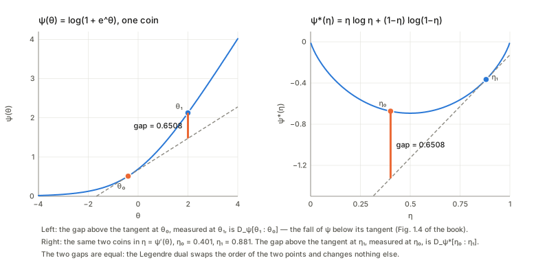
A picture first. Draw a convex function \psi and its tangent line at a point \theta_0. The curve stays above the line. The vertical gap at another point \theta is the Bregman divergence
D_\psi[\theta:\theta_0]=\psi(\theta)-\psi(\theta_0)-\nabla\psi(\theta_0)\cdot(\theta-\theta_0).
It is \ge0 by convexity, and it is zero only at \theta=\theta_0 if \psi is strictly convex. Taylor-expanding \psi about \theta_0 shows D_\psi[\theta_0+d\theta:\theta_0]=\tfrac12d\theta^\top\nabla^2\psi(\theta_0)\,d\theta+O(|d\theta|^3), so the metric of §2 is the Hessian, g_{ij}=\partial_i\partial_j\psi (1.86).
Strict convexity caveat. The book states that a smooth function is convex exactly when its Hessian is positive-definite. Strictly, positive semi-definite is the criterion for convex, and positive-definite is sufficient for strictly convex but not necessary. \psi(x)=x^4 is strictly convex, so D[x{:}0]=x^4=0.0625 at x=0.5 is positive, yet its Hessian 12x^2 is zero at x=0. Then criterion (3) of Definition 1.1 (a positive-definite g) fails at that point: you get a divergence-like gap but not a Riemannian metric there. What the construction actually needs is \nabla^2\psi\succ0 everywhere.
Examples (1.37)–(1.50).
- \psi=\tfrac12\|\xi\|^2 gives D=\tfrac12\|\xi-\xi_0\|^2 and g=I: ordinary Euclidean geometry.
- \psi=-\sum\log\xi_i on positive vectors gives D=\sum[\log\frac{\xi'_i}{\xi_i}+\frac{\xi_i}{\xi'_i}-1] (1.48), the Itakura–Saito divergence of audio processing. At random points the Bregman definition and this closed form agree (0.601510 both).
- \varphi=\sum\xi_i\log\xi_i gives the generalised KL (1.31); on probability vectors, plain KL (0.094608 both ways in my check). Negative entropy is convex, which is why KL is a Bregman divergence at all.
- Exponential family (1.39–1.58), the example that carries the whole book. A distribution of the form p(x;\theta)=\exp\{\theta\cdot x+k(x)-\psi(\theta)\} has a normaliser \psi(\theta)=\log\int e^{\theta\cdot x+k(x)}dx. For softmax, x is the indicator vector of classes 1 and 2 and \psi is log-sum-exp.
Why \psi is convex, and what its derivatives are. Differentiate the normalisation \int p(x;\theta)\,dx=1 with respect to \theta_i: \int(x_i-\partial_i\psi)\,p\,dx=0, so \nabla\psi(\theta)=\mathbb E_\theta[x] (1.54), the mean of the sufficient statistic. Differentiate once more: \partial_i\partial_j\psi=\mathbb E[(x_i-\bar x_i)(x_j-\bar x_j)], the covariance matrix (1.56), which is positive-definite because a covariance is. So \psi is convex and its Hessian is the covariance. Checks: for the softmax at \theta=(0.4,-0.8) the finite-difference gradient (0.507224,0.152773) equals the mean of the class indicators, and the Hessian \left[\begin{smallmatrix}0.24995&-0.07749\\-0.07749&0.12943\end{smallmatrix}\right] equals their covariance, entry by entry.
The Gaussian, as promised. With x=(x,x^2) the natural parameters are \theta=(\mu/\sigma^2,-1/(2\sigma^2)), \psi(\theta)=-\theta_1^2/(4\theta_2)+\tfrac12\log(-\pi/\theta_2), and \nabla\psi=(\mu,\mu^2+\sigma^2): the moment coordinates of §1.1 are the dual coordinates. At (\mu,\sigma)=(1,2), \nabla\psi=(1,5) and the Hessian is \left[\begin{smallmatrix}4&8\\8&48\end{smallmatrix}\right], matching the covariance of (x,x^2) by quadrature (\operatorname{Var}x=\sigma^2=4, \operatorname{Cov}(x,x^2)=2\mu\sigma^2=8, \operatorname{Var}x^2=2\sigma^4+4\mu^2\sigma^2=48).
Bregman divergence of an exponential family = KL, with the arguments reversed. The book says “after careful calculation”; here it is in two lines. Since \log p(x;\theta')-\log p(x;\theta)=(\theta'-\theta)\cdot x-\psi(\theta')+\psi(\theta),
\mathrm{KL}[p_{\theta'}\Vert p_\theta]=\mathbb E_{\theta'}\big[(\theta'-\theta)\cdot x\big]-\psi(\theta')+\psi(\theta) =\psi(\theta)-\psi(\theta')-\nabla\psi(\theta')\cdot(\theta-\theta')=D_\psi[\theta{:}\theta'],
using \mathbb E_{\theta'}[x]=\nabla\psi(\theta'). So D_\psi[\theta{:}\theta']=\mathrm{KL}[p_{\theta'}\Vert p_\theta] (1.57–1.58). Numerically, for softmax logits \theta=(0.4,-0.8) and \theta'=(-0.5,0.9): D_\psi[\theta{:}\theta']=0.570189, \mathrm{KL}[p_{\theta'}\Vert p_\theta]=0.570189 and the other order 0.520678. For the Gaussians N(1,2^2) and N(-0.5,1.2^2) the Bregman value 0.472076 equals the KL by quadrature. Keep this reversal in mind; it decides which projection minimises which KL in §6.
4. The Legendre dual: slopes as coordinates (§1.4)
Idea. Because \nabla^2\psi\succ0, the slope map \theta\mapsto\eta=\nabla\psi(\theta) is one-to-one: distinct points of the graph have distinct tangent planes. So the slope can serve as a coordinate. For softmax this says that the logits and the probabilities are two names for the same point, and the map between them (softmax) is the slope map of log-sum-exp.
The dual potential. Define \psi^*(\eta)=\theta\cdot\eta-\psi(\theta) with \theta=\theta(\eta) the inverse of the slope map (equivalently \psi^*(\eta)=\max_{\theta'}\{\theta'\cdot\eta-\psi(\theta')\}, the usual definition, because the maximiser has slope \eta). Differentiate with respect to \eta:
\nabla\psi^*(\eta)=\theta+\frac{\partial\theta}{\partial\eta}\eta-\nabla\psi(\theta)\frac{\partial\theta}{\partial\eta}=\theta ,
because the last two terms cancel when \nabla\psi(\theta)=\eta. So the map is symmetric: \eta=\nabla\psi(\theta) and \theta=\nabla\psi^*(\eta) (1.64). Differentiating again, \nabla^2\psi^*=\partial\theta/\partial\eta, the Jacobian of the inverse map, which is the matrix inverse of \partial\eta/\partial\theta=\nabla^2\psi. So G^*=G^{-1} (1.66), positive-definite, and \psi^* is convex. In the softmax example, at \theta=(0.4,-0.8): G=\left[\begin{smallmatrix}0.2499&-0.0775\\-0.0775&0.1294\end{smallmatrix}\right], G^*=\left[\begin{smallmatrix}4.9127&2.9412\\2.9412&9.4868\end{smallmatrix}\right] and their product is the identity to 10 decimals.
The dual divergence is the primal one with its arguments swapped (1.68). Write \theta_a,\theta_b for the points with dual coordinates \eta_a,\eta_b. Then
D_{\psi^*}[\eta_a{:}\eta_b]=\psi^*(\eta_a)-\psi^*(\eta_b)-\theta_b\cdot(\eta_a-\eta_b) =\psi(\theta_b)-\psi(\theta_a)-\eta_a\cdot(\theta_b-\theta_a)=D_\psi[\theta_b{:}\theta_a],
where the middle step substitutes \psi^*(\eta)=\theta\cdot\eta-\psi(\theta) at both points and the terms collapse. With \theta=(0.4,-0.8), \theta'=(-0.5,0.9) again: D_\psi[\theta{:}\theta']=0.570189=D_{\psi^*}[\eta'{:}\eta]. For one coin (\psi=\log(1+e^\theta), \theta_0=-0.4, \theta_1=2, so \eta_0=0.401 and \eta_1=0.881) the two gaps in the figure above are 0.6508 and 0.6508.
Theorem 1.1, the self-dual form. D_\psi[P{:}Q]=\psi(\theta_P)+\psi^*(\eta_Q)-\theta_P\cdot\eta_Q. Proof: substitute \psi^*(\eta_Q)=\theta_Q\cdot\eta_Q-\psi(\theta_Q) and use \eta_Q=\nabla\psi(\theta_Q); you get the definition back. This is the Fenchel–Young inequality, \psi(\theta)+\psi^*(\eta)\ge\theta\cdot\eta, with equality exactly when \eta=\nabla\psi(\theta) (the check gives 1.1\times10^{-16} at \eta'=\eta). The form is what makes the Pythagorean proof short: it separates the divergence into a term depending on \theta_P, a term depending on \eta_Q, and one bilinear pairing between them.
Examples (1.71)–(1.79).
- Euclidean \psi is its own dual (\psi^*=\tfrac12\|\xi^*\|^2, \xi^*=\xi): self-dual, so the two flat structures coincide.
- The pair \psi=-\sum\log\xi_i, \psi^*=-\sum[1+\log(-\xi^*_i)], and the pair \varphi=\sum\xi_i\log\xi_i, \varphi^*=\sum e^{\xi^*_i-1}. Both verified numerically at \xi=(0.7,1.9,0.4): -3.631112 both ways for the first, 3.000000 both ways for the second, and the gradients of the duals return \xi.
- Exponential family: \theta^*=\nabla\psi(\theta)=\mathbb E_\theta[x] is the expectation parameter, and \psi^*(\theta^*)=\int p\log p\,dx, the negative entropy (1.78). For the softmax at \theta=(0.4,-0.8), \psi^*(\eta)=-0.998131 and \sum_ip_i\log p_i=-0.998131. The dual divergence is KL in the natural order, D_{\psi^*}[\theta^*{:}\theta^{*\prime}]=\mathrm{KL}[p_\theta\Vert p_{\theta'}] (1.79).
A deep-learning reading of the whole section: logits ↔︎ probabilities is a Legendre pair, log-sum-exp ↔︎ negative entropy is its potential pair, and cross-entropy training (a KL divergence) is a Bregman divergence in one of the two charts.
5. Two flat structures and one metric (§1.5)
Two kinds of straight. Declare \theta an affine coordinate system: a curve \theta(t)=at+b is straight, an e-geodesic. Declare \eta affine too: \eta(t)=at+b is a m-geodesic. Because \theta\mapsto\eta is not linear, the two families of lines are different. The picture below shows one pair P=(0.7,0.2,0.1), Q=(0.1,0.3,0.6) joined by both, in the logit chart (left, e-geodesic straight) and the probability triangle (right, m-geodesic straight).
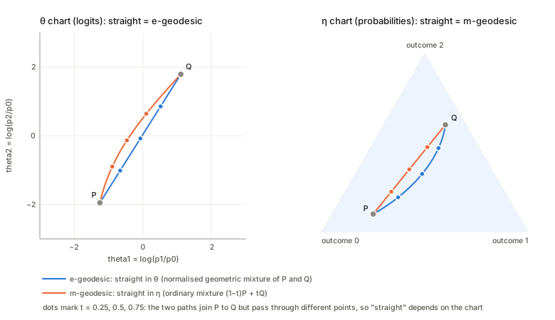
At t=0.5 the e-geodesic passes through (0.3507,0.3247,0.3247) (a normalised geometric mixture, p_i\propto\sqrt{p_iq_i}) and the m-geodesic through (0.4,0.25,0.35). Neither is the Fisher–Rao geodesic, the true shortest path for the metric G (a great-circle arc after p\mapsto\sqrt p), which passes through (0.3788,0.2821,0.3391). In this example it sits between the other two in eight of the nine coordinates I looked at (t\in\{0.25,0.5,0.75\}, three coordinates each); the exception is p_2 at t=0.75, where the three values are 0.4692 (e), 0.4750 (m) and 0.4754 (Fisher–Rao). That is the pattern one expects from the standard fact, which this chapter does not prove, that the Riemannian connection is the average of the two flat ones, but it is only an observation about one pair of points.
The metric, and the two sets of components. On the dually flat manifold, ds^2=2D_\psi[\theta{:}\theta+d\theta]=g_{ij}d\theta^id\theta^j with g_{ij}=\partial_i\partial_j\psi (1.85–1.86). The tangent vectors along the \theta-axes, e_i, are the same at every point (the chart is affine), and g_{ij}=\langle e_i,e_j\rangle. Along the \eta-axes the tangent vectors are e^{*i}, and \langle e_i,e^{*j}\rangle=\delta_i^{\,j}: the two bases are reciprocal. A vector can be written either way, A=A^ie_i=A_ie^{*i}, and the two component lists are related by A_i=g_{ij}A^j, A^i=g^{ij}A_j (1.105).
The Einstein convention, in plain words. When an index appears once up and once down in a term, sum over it. It is bookkeeping with a purpose: an up index means “how many steps along each \theta-axis”, a down index means “how much the vector registers on each \eta-axis”, and a sum of one with the other is a number that does not depend on the chart. So the length is |A|^2=A^iA_i=g_{ij}A^iA^j.
Concretely, at p=(0.5,0.3,0.2) (so \theta=(\log0.6,\log0.4)): G=\left[\begin{smallmatrix}0.21&-0.06\\-0.06&0.16\end{smallmatrix}\right] and G^*=G^{-1}=\left[\begin{smallmatrix}5.3333&2\\2&7\end{smallmatrix}\right]. A unit step along \theta_1 has components A^i=(1,0) and A_i=GA=(0.21,-0.06), so |A|^2=0.2100. The same components A^i at the point p=(0.2,0.2,0.6) give |A|^2=0.1600: parallel transport in the flat structure keeps components, not lengths, because the metric changes from place to place.
The remarkable property: orthogonality survives if you transport the two vectors by different rules. Transport A so that its A^i stay fixed (the \theta-flat rule), and B so that its B_i stay fixed (the \eta-flat rule). Then \langle A,B\rangle=A^iB_i never changes. Check: pick B with B^\top GA=0 at p=(0.5,0.3,0.2). Transporting both by the \theta rule gives \langle A,B\rangle=+0.0156 at p=(0.2,0.2,0.6), so the right angle is lost; transporting A by the \theta rule and B by the \eta rule gives 0.0. This is the algebraic reason the Pythagorean theorem needs one line of each kind.
What survives and what does not under a change of chart. The convexity of \psi is a property of the chart: re-expressing the Gaussian potential in (\mu,\sigma) gives \tilde\psi=\mu^2/(2\sigma^2)+\log\sigma+\text{const} and at (\mu,\sigma)=(0,1) the second derivative in \sigma is -1.0000<0, so it is not convex there (1.80), while it is convex in \theta. Only affine maps \theta'=A\theta+b keep it (1.81): then \psi'(\theta')=\psi(A^{-1}(\theta'-b)) is convex, the new dual coordinates are \eta'=A^{-\top}\eta (check: (-0.752257,-0.517311) both ways) and the divergence is unchanged (0.570189 both before and after). So the structure is tied to an affine class of charts, not to the manifold alone.
6. The Pythagorean theorem and projections (§1.6)
Theorem 1.2 and its proof
Let P,Q,R be three points. Suppose the m-geodesic from P to Q is orthogonal, at Q, to the e-geodesic from Q to R. Then D_\psi(R{:}P)=D_\psi(Q{:}P)+D_\psi(R{:}Q).
Proof, with the algebra written out. Expand all three divergences with the self-dual form D(X{:}Y)=\psi(\theta_X)+\psi^*(\eta_Y)-\theta_X\cdot\eta_Y and use \psi(\theta_Q)+\psi^*(\eta_Q)=\theta_Q\cdot\eta_Q (equality in Fenchel–Young at a single point). Everything collapses to
D(Q{:}P)+D(R{:}Q)-D(R{:}P)=(\theta_Q-\theta_R)\cdot(\eta_Q-\eta_P).
The m-geodesic is \eta(t)=(1-t)\eta_P+t\eta_Q with tangent \eta_Q-\eta_P; the e-geodesic is \theta(t)=(1-t)\theta_Q+t\theta_R with tangent \theta_R-\theta_Q. Orthogonality in the metric is exactly the vanishing of the pairing of one tangent given by its \eta-components with the other given by its \theta-components, which is the right-hand side. \blacksquare
Numerically, with P=(0.7,0.2,0.1), Q=(0.1,0.3,0.6) and R placed on the \theta-line through Q orthogonal to PQ, the sides hold to rounding error for every t: at t=2.2 (R=(0.1055,0.1054,0.7891)) D(Q{:}P)=1.101868, D(R{:}Q)=0.144079 and D(R{:}P)=1.24594757=D(Q{:}P)+D(R{:}Q).
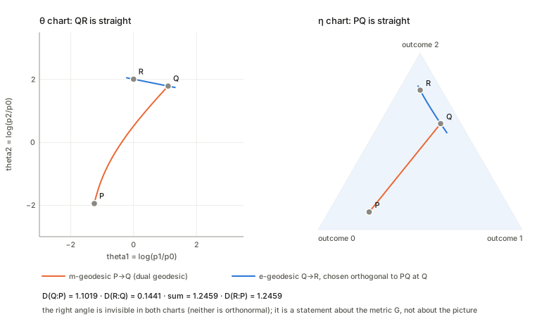
In KL language (recall D_\psi(R{:}P)=\mathrm{KL}[p_P\Vert p_R]): if the m-geodesic PQ meets the e-geodesic QR at a right angle, then \mathrm{KL}[P\Vert R]=\mathrm{KL}[P\Vert Q]+\mathrm{KL}[Q\Vert R]: here 1.245948=1.101868+0.144079. Theorem 1.3 is the mirror statement for D_{\psi^*}, with the roles of the two flat structures exchanged; it holds numerically in the same way (1.01763228 on both sides at one test, 1.09640857 at another).
A slip in the printed proof
The proof as printed states the intermediate identity (1.114) as (\theta_P-\theta_Q)\cdot(\theta^*_Q-\theta^*_R), then ends by using the orthogonality (\theta^*_P-\theta^*_Q)\cdot(\theta_Q-\theta_R)=0 of (1.119). These are not the same pairing: the algebra gives (\theta_Q-\theta_R)\cdot(\eta_Q-\eta_P), which vanishes exactly when (1.119) does, whereas the printed line pairs the wrong pairs of points in each factor. Over 200 random triples the form derived above matches D(Q{:}P)+D(R{:}Q)-D(R{:}P) to 1.1\times10^{-15}, the printed form is off by up to 13.29. Two sample triples: left side +0.431233, derived form +0.431233, printed form -0.291944; and +0.917832, +0.917832, -1.378993. The theorem is right and (1.119) is right; only the intermediate line has the indices permuted. (The interactive companion shows both forms next to the true residual.)
Projections (Theorems 1.4 and 1.5)
Given a point P and a submanifold S, the divergence from P to S is the smallest D over S (1.121). The question is where the minimum sits. The book defines the geodesic projection (the \theta-straight segment from P to a point of S meets S at a right angle) and the dual geodesic projection (the \eta-straight segment does), and claims each projection is the minimiser of one divergence.
The argument. If the \eta-straight segment from P to \hat P\in S is orthogonal to S, then for a point Q\in S very near \hat P, Theorem 1.2 applies to the triangle (P,\hat P,Q) with the m-geodesic P\hat P and a (to first order) e-direction \hat PQ. Reading off the theorem, D(Q{:}P)=D(\hat P{:}P)+D(Q{:}\hat P)\ge D(\hat P{:}P), so \hat P is a critical point of Q\mapsto D(Q{:}P).
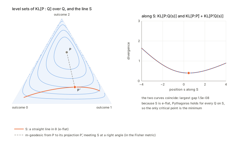
Which divergence? The printed pairing looks reversed. Theorem 1.4 as printed says the dual geodesic projection minimises D_\psi[P{:}R] (R in the second slot), and §1.6.3 pairs the geodesic projection with minimising D[P{:}Q_t] over the first slot. The argument above (and a direct derivative) says the opposite: the m-geodesic orthogonality condition is the stationarity condition of R\mapsto D_\psi[R{:}P] (variable in the first slot), because \partial_{\theta}D_\psi[\theta{:}\theta_P]=\eta(\theta)-\eta_P, whose pairing with a tangent of S is exactly the \eta-straight-segment orthogonality. I tested it on an e-flat line S in the softmax simplex: the minimiser of D_\psi[R{:}P] (equivalently \mathrm{KL}[P\Vert R]) is at s=0.458597, where the \eta-straight segment is orthogonal to S (residual -1.9\times10^{-9}) and Pythagoras holds along all of S (largest gap 8.3\times10^{-9}). The minimiser of the other order, D_\psi[P{:}R], is a different point, s=0.361703, where the \theta-straight segment is the orthogonal one, and there Pythagoras fails on this S by up to 0.215. So, for a flat S (straight in \theta): the dual-geodesic (m-) projection minimises D_\psi[R{:}P]=\mathrm{KL}[P\Vert R]. Equivalently, the e-geodesic projection minimises D_\psi[P{:}R]=\mathrm{KL}[R\Vert P] and needs S dual flat to be exact. Theorem 1.5’s pairing (flat S ↔︎ dual projection) is consistent with this; Theorem 1.4’s sentence and the em-algorithm paragraph pair projections with the other slot. I treat that as a notational inversion in the printed text rather than a mistake in the mathematics, but I flag it because every later use (maximum likelihood as an m-projection, Chapter 2) depends on getting it right.
Theorem 1.5 (flatness removes the ambiguity). If S is e-flat (straight in \theta), the m-projection of P onto S is unique and is the global minimiser of \mathrm{KL}[P\Vert R] over S. The reason is the exact Pythagoras: for every Q\in S, the e-geodesic from \hat P to Q stays inside S (it is a \theta-line) and meets P\hat P at a right angle, so D(Q{:}P)=D(\hat P{:}P)+D(Q{:}\hat P) with the last term >0 unless Q=\hat P. The dual statement holds for m-flat S and the e-projection.
Worked examples (all in the notes’ script):
- Independence model. For the 2×2 table P=\left[\begin{smallmatrix}0.4&0.1\\0.2&0.3\end{smallmatrix}\right] the independent distributions form an e-flat family (\log p_{ij}=a_i+b_j, linear in the logits). The m-projection is the product of the marginals, \left[\begin{smallmatrix}0.3&0.2\\0.3&0.2\end{smallmatrix}\right], and the minimum \mathrm{KL}[P\Vert\text{product}]=0.086305 is the mutual information. A brute-force search over product distributions finds the same minimum 0.086305, and the Pythagorean identity holds for 2000 random products to 8.9\times10^{-16}: at the product \tfrac12\otimes\tfrac12, 0.106440=0.086305+0.020136.
- Dual case. Among joints with the marginals (0.5,0.5) and (0.6,0.4) (an m-flat line), the closest to the product (0.7,0.3)\otimes(0.2,0.8) in \mathrm{KL}[Q\Vert p] is at Q_{00}=0.3000, with value 0.469085, and \mathrm{KL}[R\Vert p]=\mathrm{KL}[R\Vert\hat Q]+\mathrm{KL}[\hat Q\Vert p] over 500 random R to 3.3\times10^{-16}.
- Three-outcome picture. P=(0.15,0.25,0.60) projected onto an e-flat line: \hat P=(0.2718,0.5342,0.194), \mathrm{KL}[P\Vert\hat P]=0.398369. The profile of \mathrm{KL}[P\Vert Q(s)] along S and the sum \mathrm{KL}[P\Vert\hat P]+\mathrm{KL}[\hat P\Vert Q(s)] lie on top of each other (largest gap 1.5\times10^{-8}, limited by the minimiser’s tolerance).
Orthogonality is necessary, not sufficient
The projection theorem only says that the foot point is a critical point. The book notes this. A concrete case: in the Euclidean setting (\psi=\tfrac12\|\xi\|^2) take S the unit circle and P=(0.5,0). Both (1,0) and (-1,0) have the segment to P orthogonal to the circle (residuals 0 and 6\times10^{-17}), with D=0.125 at the first (the closest point) and D=1.125 at the second (the farthest). Flatness of S is what excludes this.
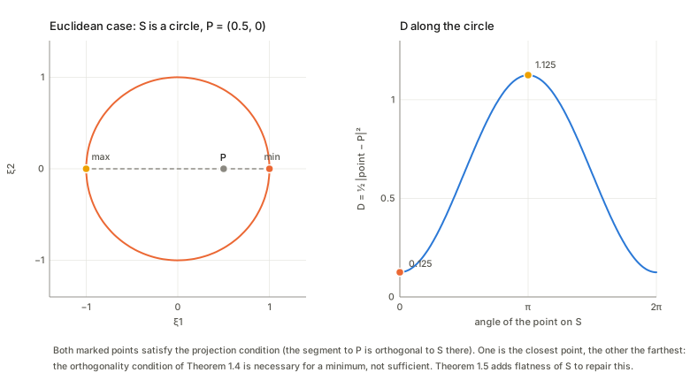
The interactive page lets you see the non-Euclidean version: for a curved arc and \mathrm{KL}[R\Vert P], put P near the centre of curvature and the divergence along the arc has two minima and a maximum.
Alternating minimisation: the em algorithm (1.123–1.124)
For two submanifolds K and S, the divergence between them is the smallest D[P{:}Q] over P\in K, Q\in S. Start from any Q_0\in S. Move P_t to the point of K closest to Q_t, then Q_{t+1} to the point of S closest to P_t. Each step cannot raise the divergence, so the sequence is non-increasing and bounded below by 0, hence the values converge:
D[P_{t-1}{:}Q_t]\ \ge\ D[P_t{:}Q_t]\ \ge\ D[P_t{:}Q_{t+1}] .
That is the whole proof of (1.124); it gives convergence of the divergence values, not of the points. When the projections are exact (flatness as above), each step has a unique solution, which is the book’s uniqueness remark. Whether the limit is the global minimum of the joint problem needs more: the joint problem is not convex in general.
Example in the KL orientation (minimise \mathrm{KL}[P\Vert Q], P\in K, Q\in S): K is the m-flat set \{P_{00}=P_{11}=0.4\} and S is the e-flat independence model. The projection onto K is available in closed form (P_{01}=0.2\,Q_{01}/(Q_{01}+Q_{10})), the projection onto S is the product of P_t’s marginals. The brute-force minimum is 0.192745, at P_{01}=P_{10}=0.1. Five random starts decrease monotonically at every half-step, for instance 0.23815\to0.19299\to0.19278\to\cdots\to0.192745 from the first start, and all five end at 0.192745 after 12 rounds.
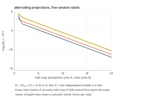
In the book’s terms the algorithm alternates an e-projection and an m-projection, hence “em” (the book introduces these names on p. 28). This is the geometric form of the EM algorithm (Chapter 8): the data manifold K is m-flat and the model S is e-flat when the full model is an exponential family.
7. Coordinates, tensors and index notation (closing remarks of §1.6)
If \zeta=f(\xi) is a new chart, line elements transform with the Jacobian, d\zeta^\kappa=J^\kappa_i\,d\xi^i (1.127), and the length ds^2 must come out the same, which forces g_{ij}=J^\kappa_iJ^\lambda_j\,g_{\kappa\lambda} (1.130). A quantity that transforms this way is a tensor. This is the formal content of “geometry does not depend on the chart”. Check on the Gaussian at (\mu,\sigma)=(1,2): the Hessian of \psi in \theta is \left[\begin{smallmatrix}4&8\\8&48\end{smallmatrix}\right]; transforming by J=\partial\theta/\partial(\mu,\sigma) gives \left[\begin{smallmatrix}0.25&0\\0&0.5\end{smallmatrix}\right]=\operatorname{diag}(1/\sigma^2,2/\sigma^2), the Fisher information of the Gaussian in (\mu,\sigma). A small step has ds^2=2.4480\times10^{-5} in either chart. So for an exponential family the Hessian metric is the Fisher metric, tied here to a concrete matrix.
The same bookkeeping gives the cleanest statement of natural gradient: because d\eta=G\,d\theta, the gradient of any function in the dual coordinates is \partial f/\partial\eta=G^{-1}\,\partial f/\partial\theta, which is exactly the natural-gradient direction in \theta. For the cross-entropy to target (0.2,0.5,0.3) at logits (0.4,-0.8): gradient in \theta is (0.00722,-0.14723) (equal to \eta- target), the gradient in \eta is (-0.39753,-1.37547), and G^{-1} times the first gives (-0.39753,-1.37547). The book’s closing argument for using coordinates (instead of coordinate-free language) is practical: choose the chart that suits the problem.
Checks of the book’s statements
| Where | Statement | What I found |
|---|---|---|
| §1.2 | the square root of a divergence is not a distance | true for KL on three coins, narrowly (2.122 vs 2.069) |
| (1.33) | trace-log-det divergence | exactly twice the Gaussian KL between N(0,P) and N(0,Q) |
| (1.34) | α-divergence on matrices | non-negative on 2000 random pairs; \alpha\to-1 gives (1.32), \alpha\to+1 gives it with arguments swapped |
| §1.3.1 | convex ⇔ Hessian positive-definite | only “⇐” for strictly convex; x^4 is strictly convex with Hessian 0 at 0 |
| (1.57–1.58) | Bregman divergence of an exponential family = KL | true, with the arguments reversed; two-line proof above |
| (1.68), (1.69) | dual divergence, self-dual form | verified; equal to 0.570189 on both sides |
| (1.80) | convexity depends on the chart | Gaussian potential has \partial^2_\sigma\tilde\psi=-1 at (0,1) |
| (1.114) | intermediate identity in the Pythagoras proof | indices permuted; the form I derive matches to 10^{-15}, the printed one is off by up to 13.29 |
| Thm 1.4, §1.6.3 | which projection minimises which divergence | printed pairing appears reversed; calculus and numerics say the m-projection minimises D_\psi[R{:}P]=\mathrm{KL}[P\Vert R] on a flat S |
| §1.6.3 | alternating minimisation, “unique when …” | the monotone decrease (1.124) holds; uniqueness is of each step, not shown for the limit |
Questions and doubts
- Existence is never discussed. Theorems 1.4–1.5 assume a point \hat P\in S with the orthogonality property exists. For an open or non-closed S it may not (the infimum sits at the boundary), and for an e-flat family in the simplex the closest point can lie on the boundary of the simplex where \theta\to\infty. The independence model avoids this because the product of marginals always exists. A clean statement needs a closedness condition on S and a steepness condition on \psi (so that the gradient map covers the whole of the dual domain). The book is explicitly not rigorous here; I would want the conditions before using the result outside exponential families.
- Does the uniqueness remark in §1.6.3 reach the limit of the algorithm? As argued above it gives unique steps. For the KL example in §6 every start reaches the same value; the joint problem there is benign. For a general flat/dual-flat pair, is the global minimum always reached? The Csiszár–Tusnády theory says yes when both sets are convex in the sense that matches each projection, but I have not checked that the geometry of this chapter delivers it. In EM for mixtures the model is not an exponential family, and local optima are the norm.
- Is the reversed pairing in Theorem 1.4 a typo or a convention? I found no reading of “geodesic” and “dual geodesic” under which the printed pairing is consistent with Theorems 1.2–1.3, so I take it as an inversion. It would be worth checking whether the corrected edition or later chapters (§2.8, maximum likelihood as m-projection) use the corrected pairing silently.
- The metric is \nabla^2\psi by definition, but Fisher information by theorem — only for exponential families. For a general convex \psi there is no statistical model behind it, and the chapter’s “converse” (every dually flat structure comes from a convex potential, announced on the last pages) is only promised. I would like to see what restrictions are needed on the manifold (simple connectivity? global affine charts?) for the potential to exist globally.
- How much freedom is there? A different \psi on the same manifold gives a different dually flat structure. Given the manifold of 3-outcome distributions, log-sum-exp is one choice; the Euclidean \tfrac12\|\xi\|^2 in the probabilities is another. Are there principled reasons to prefer one beyond “it is the exponential family”? Chapter 3 (the Fisher metric as the unique invariant one) and Chapter 4 (KL is the only invariant flat divergence) answer this; here it is only asserted by example.
- “Straight” vs “shortest”. The chapter is careful to say a geodesic here is a straight line in an affine chart and not a minimiser of length. The Fisher–Rao geodesic is a third curve. The book never says which of the three is the right path between two distributions for a given purpose (interpolating models, averaging experts, path-based training). In the softmax example the three midpoints differ in the second decimal place, which could matter for model averaging; which one is “right” depends on whether you average probabilities or logits.
- Where does the deep-learning loss live? Cross-entropy training minimises \mathrm{KL}[\text{data}\Vert\text{model}], the divergence with the model in the second slot. In this chapter’s language that is D_\psi[\theta_{\text{model}}{:}\theta_{\text{data}}] with the model in the first slot, and the minimiser is the dual (m-)projection of the data point onto the model family. Chapter 2 makes this precise; the printed pairing above is the thing to watch.
Takeaways
- One convex function builds everything. D_\psi (the gap above the tangent), \eta=\nabla\psi (the second chart), G=\nabla^2\psi (the metric), \psi^* (the dual potential), and the two flat structures are all read off \psi.
- For an exponential family \psi is log-partition, \nabla\psi is the mean, \nabla^2\psi is the covariance (= Fisher), \psi^* is the negative entropy, and D_\psi[\theta{:}\theta']=\mathrm{KL}[p_{\theta'}\Vert p_\theta] with the arguments reversed. For softmax: logits ↔︎ probabilities.
- Two straight lines, one metric. e-geodesics are straight in \theta, m-geodesics in \eta, the Fisher–Rao geodesic is neither. Transporting one vector by each rule preserves orthogonality.
- Pythagoras: m-segment \perp e-segment \Rightarrow D(R{:}P)=D(Q{:}P)+D(R{:}Q), exactly; the residual for a non-right angle is (\theta_Q-\theta_R)\cdot(\eta_Q-\eta_P).
- Projection onto a flat family is unique and optimal; for a curved family the orthogonality condition only finds critical points. The m-projection onto an e-flat family minimises \mathrm{KL}[P\Vert R] (maximum likelihood, mutual information); the e-projection onto an m-flat family minimises \mathrm{KL}[R\Vert P].
- Alternating projections lower the divergence monotonically, which is the geometry of EM and iterative scaling.
- Watch the argument order whenever the book says “projection”: derive which slot varies, as in §6, before trusting a label.
| Term | One line |
|---|---|
| Bregman divergence | D_\psi[\theta{:}\theta_0]=\psi(\theta)-\psi(\theta_0)-\nabla\psi(\theta_0)\cdot(\theta-\theta_0): gap above the tangent |
| Metric | g_{ij}=\partial_i\partial_j\psi; ds^2=2D |
| Legendre pair | \eta=\nabla\psi(\theta), \theta=\nabla\psi^*(\eta), \psi+\psi^*=\theta\cdot\eta along the graph |
| Dual metric | G^*=G^{-1} |
| Dual divergence | D_{\psi^*}[\eta_a{:}\eta_b]=D_\psi[\theta_b{:}\theta_a] |
| Self-dual form | D[P{:}Q]=\psi(\theta_P)+\psi^*(\eta_Q)-\theta_P\cdot\eta_Q |
| Exponential family | \nabla\psi=\mathbb E[x], \nabla^2\psi=\operatorname{Cov}[x], D_\psi[\theta{:}\theta']=\mathrm{KL}[p_{\theta'}\Vert p_\theta] |
| Pythagoras | m\perp e at Q: D(R{:}P)=D(Q{:}P)+D(R{:}Q); residual (\theta_Q-\theta_R)\cdot(\eta_Q-\eta_P) |
| Projection | on an e-flat S, the m-projection minimises D_\psi[R{:}P]=\mathrm{KL}[P\Vert R], uniquely |
| em algorithm | alternate the two projections; D never increases |