On the Lipschitz Continuity of Set Aggregation Functions and Neural Networks for Sets
Links
- ICLR 2026 poster page: the venue page.
- arXiv:2505.24403:
the preprint;
pdf_urlpoints here. The ICLR camera-ready is the version annotated below (44 pages, proofs in Appendix B). - Interactive companion: drag two point sets around and watch all three distances and all nine ratios update; push each of the paper’s counterexamples to its limit with a slider; and add one point to a cloud of up to 100 to see why the mean shrugs and the max jumps (Proposition 3.6).
- Runnable
code: every number on this page, and the three figures
(
python3 set_lipschitz.py --figures).make verifyruns it. - Background pages: Optimal transport, for the earth mover’s distance, couplings and Kantorovich–Rubinstein duality; Inequalities and concentration for the triangle-inequality moves.
In one paragraph
A network for sets (DeepSets, PointNet) embeds every element with an MLP, pools the embeddings with a permutation-invariant aggregator (sum, mean or max) and passes the pooled vector to a second MLP. The paper asks how much the pooled vector can move when the input set moves, that is, the Lipschitz constant of the aggregator. “Moves” needs a distance between sets, and the paper uses three: the earth mover’s distance (EMD, i.e. W_1 between the empirical distributions), the Hausdorff distance (worst nearest-neighbour gap) and a matching distance (best one-to-one pairing, with unmatched elements charged their norm). The headline result is a clean diagonal: mean is 1-Lipschitz for EMD, sum is 1-Lipschitz for matching, max is \sqrt d-Lipschitz for Hausdorff, and for sets of arbitrary size each aggregator is Lipschitz for only its own distance. When all sets have the same size M, more cells fill in (constants 1/M, M, 1). An attention-based pooling is Lipschitz for none of them. The results carry over to whole networks with the MLPs’ Lipschitz constants multiplied in, except that a bias in the first MLP breaks the sum network. Short experiments on ModelNet40 and a movie-review dataset show the bounds hold, and that accuracy drops under distribution shift track a Wasserstein distance built on the matching ground metric. Four findings below are not in the paper. The diagonal is explained by what each distance cannot see: five of the six failures are pairs of sets at distance zero whose aggregates differ. The sixth failure, max against EMD, disappears once set size is capped: the max is then Lipschitz with a constant between M and \sqrt d\,M. Attention’s failure against EMD needs unbounded inputs; on a ball it is Lipschitz. And the inequality in Proposition 3.6 is always an equality.
The spine of the argument
- Three distances (§2.4). EMD compares the sets as distributions (each element weighs 1/|X|). Hausdorff compares them as sets of locations, ignoring how many times each occurs. Matching compares them as lists to be paired, and whatever is left over is paired with the origin. Proposition 2.2 says matching is a metric away from \mathbf 0. Proposition 2.3 says matching = M\cdotEMD when both sets have M elements.
- Aggregators against distances (§3.1, Theorem 3.1). Each aggregator’s change can be written in the currency of one distance, so the triangle inequality bounds it: a transport plan for the mean, a pairing for the sum, a nearest neighbour for each coordinate of the max. For the other two distances the paper builds a family of pairs where the ratio is unbounded.
- Equal sizes (Lemma 3.2). With |X|=|Y|=M, EMD and matching are the same distance up to the factor M, so the mean, sum and max each gain a second distance. Max gains both.
- Attention (Proposition 3.3). A softmax-weighted average. A small change can shift a little weight across a large lever arm, and with unbounded inputs that is unbounded.
- Networks (§3.2, Theorem 3.4, Lemma 3.5). Composition multiplies Lipschitz constants, and a Lipschitz map moves sets by at most its constant in EMD and Hausdorff. Matching needs the map to send \mathbf 0 to \mathbf 0, which a bias prevents.
- Uses (§3.3–3.4). The distance from X to “X plus one element” (Proposition 3.6) predicts which network an outlier will hurt. A domain-adaptation bound (Theorem 3.7, from Shen et al. 2018) turns the Lipschitz constant into a statement about accuracy under shift.
Setup and notation
| Symbol | Meaning |
|---|---|
| X=\{\!\{\mathbf v_1,\dots,\mathbf v_m\}\!\} | a multiset of vectors in \mathbb R^d: order does not matter, repeats do. \{\!\{a,b\}\!\}\ne\{\!\{a,b,b\}\!\} |
| Y=\{\!\{\mathbf u_1,\dots,\mathbf u_n\}\!\} | the second multiset; sizes m=\lvert X\rvert, n=\lvert Y\rvert may differ |
| \mathcal S_{\le M}(\mathbb R^d), \mathcal S_M(\mathbb R^d) | multisets of at most M, or exactly M, vectors |
| f_{\text{SUM}}, f_{\text{MEAN}}, f_{\text{MAX}} | \sum_{\mathbf v\in X}\mathbf v; the same over \lvert X\rvert; the coordinate-wise maximum |
| d_{\text{EMD}}, d_H, d_M | earth mover’s, Hausdorff and matching distances (defined below) |
| \mathbf F | a transport plan: [\mathbf F]_{ij} is how much mass goes from \mathbf v_i to \mathbf u_j |
| \mathfrak S_m | all permutations of m items |
| \operatorname{Lip}(f) | the smallest L with \lVert f(X)-f(Y)\rVert_2\le L\,d(X,Y) for all X,Y |
| f_{\text{MLP}_1}, f_{\text{MLP}_2} | the element-wise encoder before pooling and the head after it |
| \text{NN}_g(X) | f_{\text{MLP}_2}\big(g(\{\!\{f_{\text{MLP}_1}(\mathbf v_1),\dots,f_{\text{MLP}_1}(\mathbf v_m)\}\!\})\big) with g = sum, mean or max |
| d_h | the width of f_{\text{MLP}_1}’s output, where the pooling happens (not a symbol the paper uses; see §3.2 below) |
§2.2 What “Lipschitz” measures
In plain words, a Lipschitz constant is a speed limit: if the input moves by one unit, the output moves by at most L units. For a function of one real number, it is the steepest slope the graph ever has. f(x)=3x has L=3; f(x)=\sin x has L=1; f(x)=x^2 on the whole real line has no Lipschitz constant, because its slope keeps growing. That last example will come back, because it is exactly how attention fails.
For sets the output is a vector (the pooled embedding) and distance there is Euclidean, but the input distance has to be chosen, and the choice decides the answer. Definition 2.1 is the usual one:
\lVert f(X)-f(Y)\rVert_2\;\le\;L\;d_{\mathcal X}(X,Y)\qquad\text{for all multisets }X,Y .
Two consequences are worth keeping in mind. First, if d(X,Y)=0 but f(X)\ne f(Y), no L can work, because the right side is zero. Every distance below has such pairs (they are pseudometrics), and this is the single most useful fact for reading Table 1. Second, the constant is a worst case over all pairs, including pairs a dataset would never produce. That matters for attention, and for the size cap M.
Why care: a small Lipschitz constant bounds how far an adversarial or noisy change to the input set can move the prediction (§3.3), and it enters generalisation-under-shift bounds (§3.4).
§2.4 Three ways to say how far apart two multisets are
Earth mover’s distance: sets as piles of sand
Think of X as a pile of sand: m small heaps of weight 1/m each, one at every \mathbf v_i. Y is another pile with heaps of weight 1/n at the \mathbf u_j. The EMD is the least total work, in weight × distance, needed to reshape the first pile into the second. A transport plan \mathbf F records how much sand moves from each \mathbf v_i to each \mathbf u_j:
d_{\text{EMD}}(X,Y)=\min_{\mathbf F\ge 0}\;\sum_{i=1}^m\sum_{j=1}^n[\mathbf F]_{ij}\,\lVert\mathbf v_i-\mathbf u_j\rVert_2 \quad\text{subject to}\quad \sum_j[\mathbf F]_{ij}=\tfrac1m,\;\;\sum_i[\mathbf F]_{ij}=\tfrac1n .
The first constraint says every heap of X is emptied completely, the second that every heap of Y is filled exactly. This is the Wasserstein-1 distance between the two empirical distributions (the optimal transport page builds it up from scratch). Because only the proportions matter, EMD cannot tell X from X with every element duplicated: \{\!\{\mathbf v\}\!\} and \{\!\{\mathbf v,\mathbf v\}\!\} are the same distribution, so their EMD is 0.
Hausdorff distance: sets as locations
For each point of X, find its nearest neighbour in Y; h(X,Y) is the worst such gap. Do the same from Y’s side and take the larger:
h(X,Y)=\max_{i}\min_{j}\lVert\mathbf v_i-\mathbf u_j\rVert_2,\qquad d_H(X,Y)=\max\big(h(X,Y),\,h(Y,X)\big).
d_H is small exactly when every point of either set has a close partner in the other. It looks only at where points are, never at how many sit there, so Hausdorff cannot see multiplicity at all: d_H(\{\!\{a,b\}\!\},\{\!\{a,b,b\}\!\})=0. It is also dominated by a single worst point, which is why one outlier makes it large (§3.3).
Matching distance: sets as lists to be paired, with a phantom origin
Pair the elements one to one as cheaply as possible, paying \lVert\mathbf v-\mathbf u\rVert for each pair. If X is larger, some of its elements are left over, and each one pays its own norm \lVert\mathbf v\rVert. For m\ge n,
d_M(X,Y)=\min_{\pi\in\mathfrak S_m}\Big[\sum_{i=1}^n\lVert\mathbf v_{\pi(i)}-\mathbf u_i\rVert_2+\sum_{i=n+1}^m\lVert\mathbf v_{\pi(i)}\rVert_2\Big].
The definition reads more naturally in one line: pad the smaller multiset with copies of the zero vector until the sizes agree, then take the cheapest perfect matching. A leftover \mathbf v matched to a padded \mathbf 0 pays \lVert\mathbf v-\mathbf 0\rVert=\lVert\mathbf v\rVert, which is the second sum. (Padding more zeros on both sides changes nothing: pairing \mathbf 0 with \mathbf 0 is free, and matching a real \mathbf v and a real \mathbf u to zeros separately costs \lVert\mathbf v\rVert+\lVert\mathbf u\rVert\ge\lVert\mathbf v-\mathbf u\rVert, so it never helps.) The code checks the padded form against the literal definition on 300 random pairs (largest gap 1.8\times10^{-15}).
The padded form makes two things obvious.
- The origin is special, and it is the blind spot. Adding \mathbf 0 to a multiset costs nothing: d_M(\{\!\{\mathbf v\}\!\},\{\!\{\mathbf v,\mathbf 0\}\!\})=0. That is why Proposition 2.2 says d_M is a metric only on multisets that avoid \mathbf 0, and a pseudometric otherwise. It also means d_M is not translation-invariant when sizes differ: shifting both sets by the same vector changes what a leftover element pays.
- The triangle inequality (Proposition 2.2) is short. Pad X, Y, Z to a common size. Take the best matching X\to Z and the best Z\to Y, and compose them into a matching X\to Y. Along each chain \mathbf x\to\mathbf z\to\mathbf y, \lVert\mathbf x-\mathbf y\rVert\le\lVert\mathbf x-\mathbf z\rVert+\lVert\mathbf z-\mathbf y\rVert. Sum over chains: d_M(X,Y)\le d_M(X,Z)+d_M(Z,Y). Appendix B.1 does the same thing over six orderings of \lvert X\rvert, \lvert Y\rvert, \lvert Z\rvert with four types of term; the padding collapses all six into one case. (2000 random triples: no violation.)
One pair, three distances
The smallest example that separates everything is on the real line: X=\{\!\{0,2\}\!\} and Y=\{\!\{0,2,2\}\!\}.
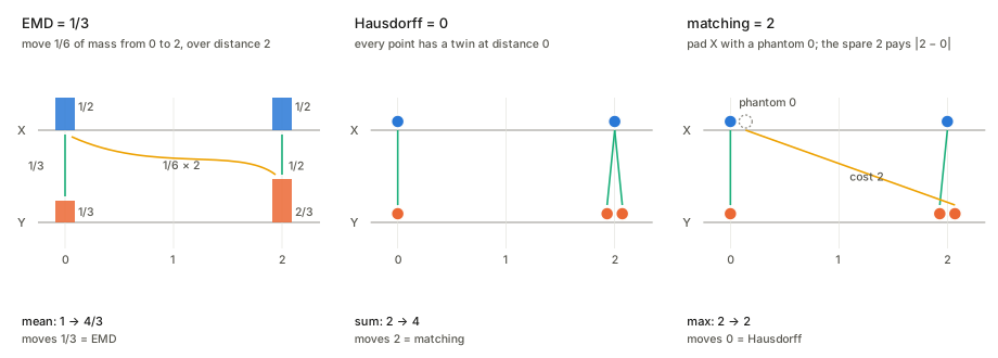
- EMD =1/3. X has half its mass at 0 and half at 2. Y has a third at 0 and two thirds at 2. Leave 1/3 at 0 and 1/2 at 2, and carry the remaining 1/6 from 0 to 2: work 1/6\times2=1/3.
- Hausdorff =0. Both sets occupy exactly the locations \{0,2\}.
- Matching =2. Pad X to \{\!\{0,2,0\}\!\}. Pair 0\leftrightarrow0 and 2\leftrightarrow2 for free; the second 2 in Y pairs with the phantom 0 and pays 2.
Now aggregate. The mean moves from 1 to 4/3, by 1/3, which is exactly the EMD. The sum moves from 2 to 4, by 2, exactly the matching distance. The max stays at 2 and moves by 0, exactly the Hausdorff distance. That is Theorem 3.1 in one picture, with every bound attained.
Proposition 2.3: for equal sizes, matching is EMD times M
If \lvert X\rvert=\lvert Y\rvert=M, both constraints in the EMD read “rows and columns each sum to 1/M”. So M\mathbf F is a doubly stochastic matrix: non-negative, with every row and column summing to 1. The Birkhoff–von Neumann theorem says every doubly stochastic matrix is an average of permutation matrices, so the set of them is a polytope whose corners are the permutations. A linear objective over a polytope is minimised at a corner. Hence the optimal plan is a permutation scaled by 1/M: each element sends all its sand to one partner. That is a matching, and
M\,d_{\text{EMD}}(X,Y)=\min_{\pi}\sum_{i=1}^M\lVert\mathbf v_{\pi(i)}-\mathbf u_i\rVert=d_M(X,Y).
(The code checks this on 200 random pairs and also uses it in reverse: an EMD between sizes m and n is computed exactly by repeating each element of X L/m times and each element of Y L/n times, L=\operatorname{lcm}(m,n), which leaves both distributions unchanged, and solving an L\times L assignment.)
In ModelNet40 every point cloud has exactly M=100 points, so in Figure 1 the EMD row and the matching row are the same scatter plot with the horizontal axis stretched by 100. That is why their correlations are identical (0.98, 0.99, 0.67 in both rows).
What each distance cannot see
Put the three blind spots side by side. Each row is a kind of change the distance scores as zero.
| Distance | Pairs at distance 0 | Mean | Sum | Max |
|---|---|---|---|---|
| EMD | Y is X with every multiplicity scaled: \{\!\{\mathbf v\}\!\} vs \{\!\{\mathbf v,\mathbf v\}\!\} | unchanged | doubles | unchanged |
| Hausdorff | same locations, any multiplicities: \{\!\{a,b\}\!\} vs \{\!\{a,b,b\}\!\} | moves | moves | unchanged |
| Matching | Y is X plus zero vectors: \{\!\{\mathbf v\}\!\} vs \{\!\{\mathbf v,\mathbf 0\}\!\} | halves | unchanged | moves if \mathbf v has a negative entry |
An aggregator can only be Lipschitz for a distance if it ignores what that distance ignores. The bold cells are therefore failures before any calculation: each one is a pair at distance 0 with different outputs. The unbolded cells are the only candidates, and they are exactly the diagonal of Table 1 plus one more: max against EMD. That cell is the subject of a separate subsection below.
§3.1 Theorem 3.1: one distance per aggregator
Theorem 3.1 (multisets of any size up to M). (1) The mean is Lipschitz for EMD with L=1, but not for Hausdorff or matching. (2) The sum is Lipschitz for matching with L=1, but not for EMD or Hausdorff. (3) The max is Lipschitz for Hausdorff with L=\sqrt d, but not for EMD or matching.
Why the three positive results hold
Each proof writes the change in the aggregate in the currency of its distance and then applies the triangle inequality once.
Mean and EMD (Appendix B.3.1). Take the optimal plan \mathbf F^{\ast}. Row i of \mathbf F^{\ast} sums to 1/m and column j sums to 1/n, so each mean can be spread over the plan:
\frac1m\sum_i\mathbf v_i-\frac1n\sum_j\mathbf u_j =\sum_{i,j}[\mathbf F^{\ast}]_{ij}\mathbf v_i-\sum_{i,j}[\mathbf F^{\ast}]_{ij}\mathbf u_j =\sum_{i,j}[\mathbf F^{\ast}]_{ij}(\mathbf v_i-\mathbf u_j).
Taking norms and using \lVert\sum\mathbf a\rVert\le\sum\lVert\mathbf a\rVert gives \lVert\Delta\text{mean}\rVert\le\sum_{ij}[\mathbf F^{\ast}]_{ij}\lVert\mathbf v_i-\mathbf u_j\rVert=d_{\text{EMD}}. The picture: the mean is the centre of mass of the sand. Moving a bit of mass F over a displacement \mathbf u-\mathbf v shifts the centre of mass by F(\mathbf u-\mathbf v), so the centre of mass cannot travel farther than the total work done. Equality holds for two singletons, so L=1 exactly.
Sum and matching (Appendix B.3.5). Pad with zeros (which do not change a sum) and take the best pairing \pi^{\ast}. Then \sum\mathbf v_i-\sum\mathbf u_i=\sum_i(\mathbf v_{\pi^{\ast}(i)}-\mathbf u_i) over padded pairs, and the triangle inequality gives \lVert\Delta\text{sum}\rVert\le d_M. The zero-padding reading makes the fit clear: the matching distance is the sum’s own geometry. A leftover element \mathbf v changes the sum by \mathbf v and is charged \lVert\mathbf v\rVert.
Max and Hausdorff (Appendix B.3.9). Fix one coordinate k. Say the largest k-th entry in X is a, attained at some \mathbf v^{\ast}, and the largest in Y is b<a. Because h(X,Y)\le d_H, \mathbf v^{\ast} has a partner \mathbf u\in Y with \lVert\mathbf v^{\ast}-\mathbf u\rVert\le d_H, so u_k\ge a-d_H, so b\ge a-d_H. Every coordinate of the max therefore moves by at most d_H, and a vector with d coordinates each at most d_H has length at most \sqrt d\,d_H. The \sqrt d is real: take X=\{\!\{\varepsilon\mathbf e_1,\dots,\varepsilon\mathbf e_d\}\!\} and Y=\{\!\{\mathbf 0\}\!\}. Then d_H=\varepsilon but the max jumps from \mathbf 0 to (\varepsilon,\dots,\varepsilon), of length \varepsilon\sqrt d. Each coordinate’s maximum comes from a different point, and each of those points is only \varepsilon from Y. (The code: ratio 1.7321=\sqrt3 for d=3.)
Why the other six fail
The paper proves each failure with a one-parameter family: two points c\mathbf 1 and \varepsilon\mathbf 1 against one, with c large relative to \varepsilon, so that the distance is of order \varepsilon while the aggregate moves by order c. Five of those families are the blind-spot pairs of the table above in thin disguise. As \varepsilon\to0 they converge to a pair at distance exactly 0. The mean against matching, for instance, uses X=\{\!\{c\mathbf 1,\varepsilon\mathbf 1\}\!\}, Y=\{\!\{c\mathbf 1\}\!\}. As \varepsilon\to0 that is \{\!\{\mathbf v\}\!\} against \{\!\{\mathbf v,\mathbf 0\}\!\}: the phantom origin absorbs the extra element for free, while the mean is dragged halfway to it. The code evaluates all five at distance exactly 0:
| Aggregator / distance | Pair | Distance | \lVert f(X)-f(Y)\rVert |
|---|---|---|---|
| mean / Hausdorff | \{\!\{a,b\}\!\} vs \{\!\{a,b,b\}\!\}, a=(1,0), b=(0,2) | 0 | 0.3727 |
| mean / matching | \{\!\{\mathbf v\}\!\} vs \{\!\{\mathbf v,\mathbf 0\}\!\}, \mathbf v=(-1,-2) | 0 | 1.1180 |
| sum / EMD | \{\!\{\mathbf v\}\!\} vs \{\!\{\mathbf v,\mathbf v\}\!\} | 0 | 2.2361 |
| sum / Hausdorff | \{\!\{\mathbf v\}\!\} vs \{\!\{\mathbf v,\mathbf v\}\!\} | 0 | 2.2361 |
| max / matching | \{\!\{\mathbf v\}\!\} vs \{\!\{\mathbf v,\mathbf 0\}\!\} | 0 | 2.2361 |
So these five are not about constants being large. The aggregator is not even a function of the distance’s equivalence classes: two inputs the distance calls identical get different outputs. No amount of weight decay or spectral normalisation can fix that; only a different distance can.
The sixth failure, max against EMD, depends on the size cap
Here the table offers no zero-distance pair. EMD’s blind spot is duplication, and duplicating elements never changes a maximum. The paper’s witness (Appendix B.3.7) is different in kind. It takes m=\lfloor L+1\rfloor elements per set: m-1 shared elements summing to \mathbf 0, and one top element per set, the two tops 1 apart. The max moves by 1, the EMD is 1/m, and the ratio is m. To beat a proposed constant L it needs more than L elements. On \mathcal S_{\le M}(\mathbb R^d), the domain the theorem is stated on, that is not available once L\ge M.
In fact the max is Lipschitz for EMD when sizes are capped, and the argument is one line. Fix a coordinate k with a=\max_X(\cdot)_k>b=\max_Y(\cdot)_k, and let \mathbf v^{\ast} attain a. It carries mass 1/m\ge1/M, and every point of Y is at least a-b away from it (their k-th coordinates are all at most b). Emptying \mathbf v^{\ast}’s heap therefore costs at least (a-b)/m, so
a-b\;\le\;m\,d_{\text{EMD}}\;\le\;M\,d_{\text{EMD}}, \qquad\text{hence}\qquad \lVert f_{\text{MAX}}(X)-f_{\text{MAX}}(Y)\rVert\le\sqrt d\,M\,d_{\text{EMD}}(X,Y).
The witness shows the constant is at least M. So on \mathcal S_{\le M} the true constant lies in [M,\sqrt d\,M]; a hill-climbing search in d=2 never exceeded M.
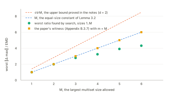
What Theorem 3.1(3) actually establishes, then, is that no constant works uniformly in the size: on multisets of unbounded size the max is not Lipschitz for EMD, but for any fixed cap it is, with a constant that grows linearly in the cap. The paper’s own Lemma 3.2 already contains half of this (the constant M for equal sizes). The same size-hungry witness is also used for sum against EMD (Appendix B.3.4), where it is harmless: the pair \{\!\{\mathbf v\}\!\}, \{\!\{\mathbf v,\mathbf v\}\!\} kills that cell for any M\ge2.
“No two of the distances are bi-Lipschitz equivalent”
Two distances are bi-Lipschitz equivalent when each is at most a constant times the other. Then any function Lipschitz for one would be Lipschitz for the other. The mean is Lipschitz for EMD but not for the other two, which separates EMD from both; the sum separates matching from Hausdorff. This is a genuine consequence for sets of mixed size. For equal sizes it is false for the pair EMD and matching (Proposition 2.3 makes them proportional).
Lemma 3.2: when every set has the same size M
With \lvert X\rvert=\lvert Y\rvert=M the matching blind spot is gone (there is nothing to pad) and EMD’s blind spot is gone (duplicating everything changes the size). Proposition 2.3 converts between EMD and matching at the rate M:
| Mean | Sum | Max | |
|---|---|---|---|
| EMD | 1 | M | M |
| Hausdorff | ✗ | ✗ | \sqrt d |
| Matching | 1/M | 1 | 1 |
- Mean/matching =1/M and sum/EMD =M are Theorem 3.1 with Proposition 2.3 substituted.
- Max/matching =1 (Appendix B.4.5) needs its own argument. For each coordinate k, the larger of the two maxima is attained at some element, which the optimal pairing matches to some partner; that coordinate’s gap is at most the gap between those two partners in coordinate k (the other side’s max is at least the partner’s entry). So every coordinate’s gap is charged to one matched pair. Within one pair, the charged coordinates’ squared gaps add up to at most that pair’s squared distance. Across pairs, \sqrt{\sum_p s_p^2}\le\sum_p s_p, and \sum_p s_p\le d_M.
- Max/EMD =M follows from max/matching and Proposition 2.3, and the B.3.7 witness shows it is tight.
- Hausdorff still fails for mean and sum, and still at distance zero: \{\!\{a,a,b\}\!\} and \{\!\{a,b,b\}\!\} have the same size, the same locations and different means.
- Not in the lemma but worth having: on \mathcal S_M, d_H\le d_M, because each point’s nearest neighbour is at least as close as its matched partner, and one pair’s distance is at most the sum of all of them. So with equal sizes the three distances are ordered d_H\le d_M=M\,d_{\text{EMD}}.
The paper’s reading, that max is the safe default for equal-size inputs because it is Lipschitz for all three distances, follows from the table. It is also the setting of Table 3’s ModelNet40 column, where the max network wins by 14 points.
Proposition 3.3: attention
The attention pooling is a softmax-weighted average:
f_{\text{ATT}}(X)=\sum_i\alpha_i\mathbf v_i,\qquad \alpha_i=\frac{\exp\big(\mathbf q^\top g(\mathbf W\mathbf v_i)\big)}{\sum_j\exp\big(\mathbf q^\top g(\mathbf W\mathbf v_j)\big)} .
Each element gets a score s(\mathbf v)=\mathbf q^\top g(\mathbf W\mathbf v), the scores are softmaxed into weights, and the output is a convex combination of the elements. With all scores equal it is the mean; with one score much larger it approaches picking that element, like a max. The proposition says there are weights \mathbf W,\mathbf q for which it is Lipschitz for none of the three distances.
The witness, with numbers
Appendix B.5 takes \mathbf W=-\mathbf I, \mathbf q=\mathbf 1, g=\text{ReLU}, so the score is s(\mathbf v)=\sum_k\max(0,-v_k): how negative the element is. Then
X=\{\!\{c\mathbf 1,\;\varepsilon\mathbf 1\}\!\},\qquad Y=\{\!\{c\mathbf 1,\;-\varepsilon\mathbf 1\}\!\}.
In X both elements are non-negative, both scores are 0, both weights are 1/2. In Y the element -\varepsilon\mathbf 1 scores d\varepsilon, so its weight rises from 1/2 to e^{d\varepsilon}/(1+e^{d\varepsilon})\approx\tfrac12+\tfrac{d\varepsilon}{4}. A weight shift of about d\varepsilon/4 between two elements that are about c\sqrt d apart moves the output by about (d\varepsilon/4)\,c\sqrt d. Meanwhile the sets differ by moving one element from \varepsilon\mathbf 1 to -\varepsilon\mathbf 1, which is an EMD of \sqrt d\,\varepsilon. Worked exactly (the code matches to four decimals), with e=\exp(d\varepsilon),
\frac{\lVert f_{\text{ATT}}(X)-f_{\text{ATT}}(Y)\rVert}{d_{\text{EMD}}(X,Y)} =\frac{c\,(e-1)+\varepsilon\,(1+3e)}{2\,(1+e)\,\varepsilon} \;\xrightarrow[\;\varepsilon\to0\;]{}\;\frac{c\,d}{4}+1 .
For fixed c this stays bounded: at c=1, d=3 it tends to 1.75 however small \varepsilon gets. It is unbounded only as c\to\infty. The failure is the x^2 kind from §2.2, not the blind-spot kind. The lever arm c is the distance between the elements the weight moves between, and the input space offers arbitrarily long lever arms.
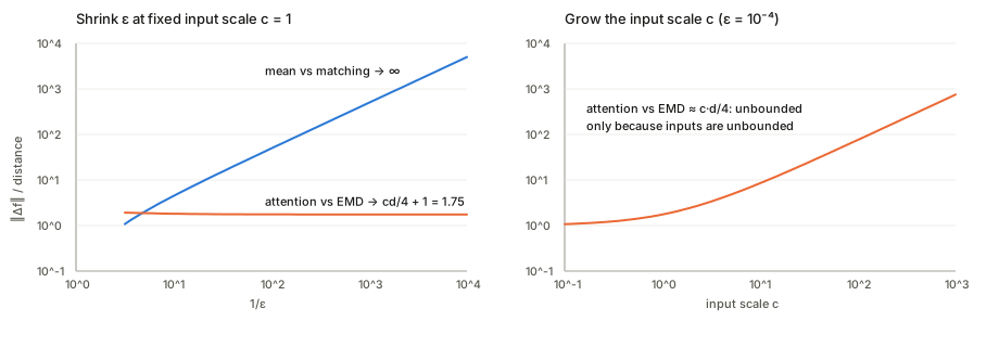
The left panel contrasts the two failure modes. The mean against matching blows up as \varepsilon\to0 at a fixed scale, because the pair converges to a blind-spot pair. Attention against EMD does not; it needs the right panel, a growing scale.
What survives on a bounded input domain
Three observations, all checked in the code, place attention next to the mean rather than below it.
- Attention ignores duplication. Duplicating every element duplicates every term in the numerator and the denominator of the softmax, so f_{\text{ATT}} is a function of the empirical distribution, exactly like the mean. It has no zero-EMD counterexample.
- On a ball it is Lipschitz for EMD. If every \lVert\mathbf v\rVert\le R, write f_{\text{ATT}}=\frac{\int\mathbf v\,w(\mathbf v)\,d\mu}{\int w(\mathbf v)\,d\mu} with w=e^{s} and \mu the empirical distribution. On the ball, w and \mathbf v\,w(\mathbf v) are Lipschitz and w is bounded below by e^{-\max\lvert s\rvert}, so numerator and denominator are Lipschitz in W_1 (by Kantorovich–Rubinstein duality, integrals of Lipschitz functions are), and so is their ratio. The constant grows with R\lVert\mathbf W\rVert\lVert\mathbf q\rVert. Search with a fixed random \mathbf W,\mathbf q in d=3: worst ratios 1.09, 1.47, 2.97 for R=1,4,16.
- Against Hausdorff and matching it fails like the mean, at distance zero: \{\!\{a,b\}\!\}\to\{\!\{a,b,b\}\!\} doubles b’s share of the softmax (the output moves by 0.53 in the code’s example), and \{\!\{\mathbf v\}\!\}\to\{\!\{\mathbf v,\mathbf 0\}\!\} gives the phantom zero some weight.
So the fair summary is: attention is mean-like. It is Lipschitz for EMD on any bounded domain (point clouds normalised to unit variance, as in Appendix D, are effectively bounded), with a constant that depends on the weights and the radius; and it fails Hausdorff and matching for the mean’s reasons. Kim et al. (2021) found the same unbounded-domain mechanism in dot-product self-attention.
\ell_2 attention (Appendix B.6)
Replacing the score by -\lVert\mathbf q-g(\mathbf W\mathbf v)\rVert (the construction Kim et al. use to make self-attention Lipschitz) does not help here, and the same witness works. One sign is off in B.6.1–B.6.2: with the printed \mathbf q=(-\varepsilon,\dots,-\varepsilon), the weights in Y come out as (0.586,0.414), the reverse of the printed ones. With \mathbf q=(+\varepsilon,\dots,+\varepsilon) they are (0.414,0.586) as printed (d=3, \varepsilon=0.2). The conclusion is unaffected. Also, B.5.3 and B.6.3 end with “>L\,d_M(X,Y)” where they mean d_H.
§3.2 Theorem 3.4 and Lemma 3.5: whole networks
The network is encoder, pool, head: \text{NN}_g=f_{\text{MLP}_2}\circ g\circ f_{\text{MLP}_1}, with the encoder applied to each element. Two facts do all the work.
- Composition multiplies constants: \operatorname{Lip}(f\circ h)\le\operatorname{Lip}(f)\operatorname{Lip}(h).
- A Lipschitz map moves sets by at most its constant. Apply f=f_{\text{MLP}_1} to every element. For EMD, reuse the optimal plan for (X,Y) as a (possibly suboptimal) plan for (f(X),f(Y)): each pair’s cost shrinks by at most the factor \operatorname{Lip}(f), so d_{\text{EMD}}(f(X),f(Y))\le\operatorname{Lip}(f)\,d_{\text{EMD}}(X,Y). For Hausdorff, a nearest neighbour within r stays within \operatorname{Lip}(f)\,r. For matching, matched pairs behave the same way, but a leftover \mathbf v is now charged \lVert f(\mathbf v)\rVert, and \lVert f(\mathbf v)\rVert\le\operatorname{Lip}(f)\lVert\mathbf v\rVert+\lVert f(\mathbf 0)\rVert.
That gives Theorem 3.4: \text{NN}_{\text{MEAN}} is Lipschitz for EMD with constant at most \operatorname{Lip}(f_{\text{MLP}_2})\operatorname{Lip}(f_{\text{MLP}_1}), and \text{NN}_{\text{MAX}} for Hausdorff with \sqrt{\cdot}\,\operatorname{Lip}(f_{\text{MLP}_2})\operatorname{Lip}(f_{\text{MLP}_1}). For \text{NN}_{\text{SUM}} and matching the same steps give a Lipschitz bound plus an offset:
\lVert\text{NN}_{\text{SUM}}(X)-\text{NN}_{\text{SUM}}(Y)\rVert \le\operatorname{Lip}(f_{\text{MLP}_2})\Big(\operatorname{Lip}(f_{\text{MLP}_1})\,d_M(X,Y)+\big\lvert\lvert X\rvert-\lvert Y\rvert\big\rvert\,\lVert f_{\text{MLP}_1}(\mathbf 0)\rVert\Big).
The bias breaks the sum network
The offset is the whole story of Theorem 3.4(2). The encoder’s bias makes f_{\text{MLP}_1}(\mathbf 0)\ne\mathbf 0, so the phantom zero that the matching distance adds for free is encoded as a real vector and summed in. The paper’s witness (Appendix B.7.2) is one-dimensional: f_1(x)=\text{ReLU}(a_1x+b_1), f_2(x)=a_2x+b_2, X=\{\!\{c,c\}\!\}, Y=\{\!\{c\}\!\}. With a_1=a_2=1, b_1=0.5:
| c | d_M(X,Y) | output change | ratio |
|---|---|---|---|
| 0.1 | 0.100 | 0.600 | 6 |
| 0.01 | 0.010 | 0.510 | 51 |
| 0.001 | 0.001 | 0.501 | 501 |
The output change never drops below b_1=0.5, while the distance goes to zero. Remove the bias (or any other way of ensuring f_{\text{MLP}_1}(\mathbf 0)=\mathbf 0) and the offset vanishes; the code checks a bias-free ReLU encoder against the bound \operatorname{Lip}\cdot\operatorname{Lip}=13.8 and finds at most 4.8. With equal sizes the offset vanishes too, which is Lemma 3.5(2).
The \sqrt d in the max network is the hidden width
In Appendix B.7.3 the \sqrt d comes from applying Theorem 3.1(3) to the encoded multisets f_{\text{MLP}_1}(X), whose elements live in the encoder’s output space \mathbb R^{d_h}. So the constant is \sqrt{d_h}\,\operatorname{Lip}(f_{\text{MLP}_2})\operatorname{Lip}(f_{\text{MLP}_1}), not \sqrt d with d the input dimension that the theorem statement’s notation suggests. This is not cosmetic. In the experiments d=3 (ModelNet40) but d_h=64, a factor of 8/\sqrt3\approx4.6.
A counterexample to the bound read with the input dimension: a one-dimensional input, and an encoder with 16 outputs, each a tent of height 1 and slope 1 centred at 0,3,6,\dots,45. The tents do not overlap, so \operatorname{Lip}(f_{\text{MLP}_1})=1. Let X be the 16 centres and Y the centres shifted by 0.25. Then d_H(X,Y)=0.25 and every coordinate of the max drops from 1 to 0.75, so the pooled vector moves by 0.25\sqrt{16}=1. The bound with d=1 says 0.25; with d_h=16 it says 1, attained.
§3.3 Stability: adding one element (Proposition 3.6)
A natural perturbation of a point cloud or a document is one extra element \mathbf w. For the mean network the relevant quantity is the EMD from X to X'=X\cup\{\!\{\mathbf w\}\!\}; for the max network, the Hausdorff distance.
Hausdorff. Every old point is in both sets, so the only nonzero nearest-neighbour gap is the new point’s: d_H(X,X')=\min_i\lVert\mathbf v_i-\mathbf w\rVert. One outlier far from the cloud makes it as large as its distance to the cloud.
EMD, and why the bound is an equality. As a distribution, X' is a mixture: with t=1/(n+1),
\mu_{X'}=(1-t)\,\mu_X+t\,\delta_{\mathbf w}.
To turn X into X' a fraction t of the sand has to end up at \mathbf w. The paper’s plan takes it evenly from every heap, and bounds the EMD by the cost of that plan, \frac{1}{n(n+1)}\sum_i\lVert\mathbf v_i-\mathbf w\rVert. Taking it evenly is optimal, so the bound is always an equality. The cleanest argument is Kantorovich–Rubinstein duality, which writes W_1(\mu,\nu)=\sup_\varphi\big(\int\varphi\,d\mu-\int\varphi\,d\nu\big) over all 1-Lipschitz functions \varphi (the optimal transport page explains why). Here \mu_X-\mu_{X'}=t(\mu_X-\delta_{\mathbf w}), so every test function sees exactly t times the difference between X and the single point \mathbf w. Hence W_1(\mu_X,\mu_{X'})=t\,W_1(\mu_X,\delta_{\mathbf w}). The distance to a single point is easy, because all the sand must go there: W_1(\mu_X,\delta_{\mathbf w})=\frac1n\sum_i\lVert\mathbf v_i-\mathbf w\rVert. So
d_{\text{EMD}}(X,X')=\frac{1}{n(n+1)}\sum_{i=1}^n\lVert\mathbf v_i-\mathbf w\rVert\quad\text{exactly}.
The code confirms the equality on 200 random cases (largest gap 4\times10^{-16}); the paper names only the trivial equality case where every point coincides.
The two formulas explain Table 2. With n=100 Gaussian points and a new point at 1.5\times the farthest one, the EMD change is 0.047 and the Hausdorff change 1.55, thirty times larger. The paper’s Pert. #1 (add the highest-norm element found in the dataset) costs the mean network 2 points of accuracy and the max network 20. Pert. #2 (add \mathcal U(0,0.2)^d noise to every element) moves every element a little, and there the max network is the robust one (4.8 against 13.6). The theory does not predict this one. Proposition C.2 gives the EMD and the Hausdorff distance the same bound, k\sqrt d, so the difference has to come from the trained networks’ constants or from the data, not from the choice of distance. Appendix E.3 frames the outlier result the same way: the perturbed cloud is on average 2.63 farther from its original, in Hausdorff distance, than the other clouds of its class are.
§3.4 Generalisation under distribution shift (Theorem 3.7)
The bound is borrowed from Shen et al. (2018), itself a Wasserstein version of Ben-David et al. (2010). For a binary task with source and target input distributions \mu_S, \mu_T and a hypothesis class whose members are all L-Lipschitz,
\epsilon_T(h)\;\le\;\epsilon_S(h)+2L\,W_1(\mu_S,\mu_T)+\lambda,
where \epsilon_S,\epsilon_T are the source and target errors and \lambda is the combined error of the best single hypothesis on both. In words: moving the data by W_1 can change a prediction by at most L per unit moved, and the two factors of the bound are exactly that.
The new ingredient is what W_1 means when each input is a multiset. The inputs are points of a metric space whose metric is EMD (for \text{NN}_{\text{MEAN}}) or Hausdorff (for \text{NN}_{\text{MAX}}), and W_1(\mu_S,\mu_T) is optimal transport between distributions of multisets with that ground metric. With EMD as the ground metric it is a Wasserstein distance whose cost is itself a Wasserstein distance: transport of documents, each of which is a pile of words. The paper does not have to prove anything new here. It only needs the Lipschitz constant, and §3.2 supplies it for exactly the two networks.
Experiments, briefly
- Aggregators alone (Figure 1, Polarity in Figure 4). The latent multisets just before pooling (100 points in \mathbb R^{64} per ModelNet40 cloud) are compared pairwise, 4,950 pairs. Every dot is below its bound. Mean against EMD is close to tight; max against Hausdorff is loose. The EMD and matching rows are the same data rescaled by M=100 (see Proposition 2.3 above).
- Networks (Figure 2, Figure 5). One linear layer, pool, one linear layer, so \operatorname{Lip} is a product of two spectral norms and exact. Bounds hold and are loose for sum and very loose for max.
- Stability (Table 2). Discussed under Proposition 3.6.
- Size shift (Figure 3). 2,000 Polarity documents are sorted by length into 10 bins of 200. A network trained on the shortest bin is tested on the others. The accuracy drop and W_1 between bins correlate at r\approx0.9. Amazon reviews across four product domains (Figure 7): r=0.917 for mean/EMD and 0.941 for max/Hausdorff.
- Plain accuracy (Table 3). Max wins on ModelNet40 (77.2 vs 63.4 and 60.1) and Polarity, mean on IMDB regression, sum on IMDB-BINARY (multisets of node degrees, where counts matter).
Questions and doubts
- Theorem 3.1(3)’s “max is not Lipschitz for EMD” needs unbounded sizes, although the theorem is stated on \mathcal S_{\le M}. The witness needs \lfloor L+1\rfloor elements. For a fixed cap M the max is Lipschitz with a constant in [M,\sqrt d\,M] (above). The correct statement is “no constant uniform in M”, which is also what Table 1’s footnote implies. The same large-m witness is used for sum/EMD, where a two-element witness would do.
- Five of the six negative results are about pseudometric blind spots, not about magnitude. The paper proves them with c-versus-\varepsilon families, which reads as “the constant is very large”. In fact the aggregator gives different answers on pairs the distance calls identical. Put that way, the guideline in §5 becomes sharper. Choosing an aggregator is choosing what to be blind to: duplication (mean), multiplicity (max) or zero vectors (sum).
- Attention’s non-Lipschitzness for EMD is an unbounded-domain effect. On any ball it is Lipschitz, with a constant that depends on the ball and on \mathbf W,\mathbf q. The practical worry is then how large that constant gets for trained weights, a question the paper does not measure. Figure 6’s lower correlations do not bear on the question either way. A function can be Lipschitz and poorly correlated with a distance, or correlated and not Lipschitz.
- \sqrt d versus \sqrt{d_h} in Theorem 3.4(3) and Figure 2’s max line. Which d the dashed line in Figure 2 uses is not stated. The dots sit far below it either way.
- Proposition 3.6(1) is an equality. It should also be the formula quoted in Appendix E.3, where the EMD analysis of Pert. #1 is done numerically.
- The matching distance is anchored to the origin. Leftover elements pay their norm, so the distance depends on where \mathbf 0 is. Point clouds are centred in Appendix D, which makes that choice sensible for inputs. In a hidden layer after a ReLU and a bias, where the origin sits is up to the network. The bias failure of \text{NN}_{\text{SUM}} is this issue in another form.
- The generalisation bound is not evaluated, only correlated. In Figure 7, W_1 is between 2 and 2.4 with the EMD ground metric (about 4 with Hausdorff), and the Lipschitz bounds of comparable networks in Figures 2 and 5 are far above 1. So 2LW_1 exceeds 1, and as a bound on a 0–1 error the theorem is vacuous. Figure 3’s correlation is over 10 bins whose W_1 and accuracy drop both grow with distance from the training bin. Nearly any quantity that grows with document length would correlate as well.
- Hypotheses into \{0,1\} are not Lipschitz unless constant on connected pieces of the input space. Theorem 3.7 needs real-valued outputs (probabilities), and the reported accuracies come from thresholding them. The step is standard, but it means the bound is about the soft output.
- Small slips. The \ell_2-attention witness’s \mathbf q has the wrong sign; B.5.3 and B.6.3 end with d_M for d_H; B.7.1 says the network’s constant is upper bounded by “\operatorname{Lip}\operatorname{Lip}\,d_{\text{EMD}}(X,Y)” (the distance should not be in a constant).
Takeaways
- Each aggregator has a native geometry. Mean is the centre of mass, so it lives with transport (EMD). Sum adds leftover elements at face value, so it lives with padded matching. Max looks only at extreme locations, so it lives with Hausdorff. The Lipschitz constants 1, 1 and \sqrt d are each one triangle inequality.
- Before computing any constant, check the blind spots. If a distance scores two different inputs as zero apart and the function separates them, the function is not Lipschitz for that distance, whatever its weights. That settles five of Table 1’s six failures at a glance.
- Size caps and input bounds change the answers. Max against EMD, and attention against EMD, are both Lipschitz once set size, or input norm, is bounded. The constant grows with the bound. The “✗” entries in the paper mix these with the blind-spot failures, which are unconditional.
- For networks, biases matter only for the sum. Lipschitz maps push EMD and Hausdorff forward cleanly. Matching also needs f(\mathbf 0)=\mathbf 0, and the max bound’s \sqrt{\cdot} is the width of the pooled layer.
- One outlier is cheap in EMD and expensive in Hausdorff, exactly \frac{1}{n(n+1)}\sum_i\lVert\mathbf v_i-\mathbf w\rVert against the nearest-neighbour distance. That is the whole mechanism behind the mean network’s robustness to outliers and the max network’s fragility to them.