Fine-Tuning can Distort Pretrained Features and Underperform Out-of-Distribution
Links
- OpenReview forum: the ICLR 2022 venue page.
- arXiv:2202.10054:
preprint, 54 pages with the appendix proofs.
make fetchpulls the PDF from here. - Interactive companion: the paper’s 2-D toy (Figure 2) as a live gradient flow. Drag the tilt of the pretrained feature and the initial head, scrub time.
- Code:
numpy only.
python3 code/feature_distortion.pyprints every number quoted below;--figuresregenerates the three SVGs. - Principal angles between subspaces: the one piece of linear algebra the main theorem is written in.
Kumar, Raghunathan, Jones, Ma and Liang, Fine-Tuning can Distort Pretrained Features and Underperform Out-of-Distribution, ICLR 2022.
In one paragraph
You have a good pretrained feature extractor and a labelled downstream set. Linear probing (LP) freezes the features and trains only the last linear layer. Fine-tuning (FT) trains everything. FT wins on test data that looks like the training data (in-distribution, ID). The paper shows that when the pretrained features are already good and the test data is far from the training data (out-of-distribution, OOD), FT loses to LP, by 7 accuracy points on average over ten benchmarks. The explanation is a piece of mechanics. The gradient on the feature extractor is built from training inputs, so the features change only in directions the training data spans and stay exactly as pretrained in every other direction. A randomly initialised head, however, is far from right, so fitting the training data forces the head and the features to move together. The head ends up tuned to the changed features, and on OOD inputs it meets the unchanged ones. Starting from a head that is already good (the linear-probed head, the LP-FT recipe) removes the need to move the features, and the distortion goes with it.
The spine of the argument
- Model: f(x)=v^\top B x with feature extractor B\in\mathbb R^{k\times d} and head v\in\mathbb R^k. Fit the training set by gradient flow on both, starting at the pretrained B_0.
- Fact 1 (Lemma A.3). B_{\mathrm{ft}}(t)\,x=B_0\,x for every x perpendicular to all training inputs. The feature extractor never moves outside the training span S.
- Fact 2 (Lemma A.4). vv^\top-BB^\top is conserved. The head and the features cannot move independently.
- To have small OOD error the head must be close to the true head v_\star (because OOD inputs only “see” the unchanged features). The conserved quantity then forces B to move a lot inside S if v_0 is far from v_\star, and that raises the ID-side error. Either way some subspace is wrong: this is Theorem 3.3.
- LP keeps the features, so its OOD error is about \epsilon\|w_\star\| (first order in the feature error \epsilon). FT’s lower bound does not go to zero with \epsilon. That gap is Theorem 3.5.
- FT can still fit the training data exactly with imperfect features, and LP cannot: Proposition 3.6.
- If the head is initialised at the LP solution and the features are perfect, the gradient is already zero and nothing moves: Proposition 3.7, the LP-FT idea.
Setup and notation
| Symbol | Meaning |
|---|---|
| d,\;k,\;m,\;n | input dimension, feature dimension, dimension of the ID subspace, number of training examples. k<m<d-k and n\ge m |
| B\in\mathbb R^{k\times d},\;v\in\mathbb R^{k} | feature extractor (a linear map) and head; predictor v^\top Bx |
| B_\star,\,v_\star,\,w_\star=B_\star^\top v_\star | ground truth (well-specified: y=w_\star^\top x); B_\star has orthonormal rows |
| B_0 | pretrained extractor, orthonormal rows, d(B_0,B_\star)\le\epsilon |
| d(B,B')=\min_U\lVert B-UB'\rVert_2 | distance between extractors up to a rotation U (rotating features is harmless: (Uv)^\top(UB)=v^\top B) |
| X\in\mathbb R^{n\times d},\;Y\in\mathbb R^n | training inputs (as rows) and labels; S=\operatorname{rowspace}(X), \dim S=m |
| S^\perp | directions perpendicular to every training input: the “never seen” part of input space |
| R_0=\operatorname{rowspace}(B_0) | the k-dimensional subspace of inputs that the pretrained features read |
| \Sigma=\mathbb E_{P_{\rm ood}}[xx^\top] | OOD second moment, assumed to reach outside S |
| \widehat L(v,B)=\lVert XB^\top v-Y\rVert_2^2 | training loss; L_{\rm ood}(v,B)=(w_\star-B^\top v)^\top\Sigma(w_\star-B^\top v) |
| \cos\theta_{\max}(R,S) | cosine of the largest principal angle (\sigma_{\min}(E^\top F) for orthonormal bases E,F) |
| \varphi^2=\lvert (v_0^\top v_\star)^2-(v_\star^\top v_\star)^2\rvert | how misaligned the initial head is with the true head |
| FT, LP, LP-FT | fine-tune everything; train head only; train head, then fine-tune from that head |
The flows are
\dot v_{\rm ft}=-\nabla_v\widehat L,\quad \dot B_{\rm ft}=-\nabla_B\widehat L,\qquad \dot v_{\rm lp}=-\nabla_v\widehat L,\quad \dot B_{\rm lp}=0,
with B_{\rm ft}(0)=B_{\rm lp}(0)=B_0 and v(0)=v_0 (random, or zero). Gradient flow is gradient descent with an infinitesimal step, so the update is a differential equation and the paper can reason about the path instead of only its endpoint.
Why the path matters
The setting is overparameterised (m<d-k and B is free to move), so many parameter settings fit the training data perfectly. Fine-tuning from a pretrained B_0 and training from scratch minimise the same loss and differ only in where they start. Which zero-loss solution gradient flow lands on depends on the whole trajectory, which is the “implicit regularisation of the initialisation”. There is no closed form for the trajectory (the problem is non-convex), so the paper avoids solving it and instead finds quantities that cannot change along it.
Result 1: the feature extractor only moves inside the training span
The gradient of \widehat L with respect to B, with residual r=XB^\top v-Y\in\mathbb R^n:
\widehat L=\lVert r\rVert^2 \;\Rightarrow\; \frac{\partial\widehat L}{\partial B_{ij}}=2\sum_{s} r_s\,v_i X_{sj} \;\Rightarrow\; \nabla_B\widehat L=2\,v\,r^\top X .
Every row of \nabla_B\widehat L is 2v_i\,r^\top X, a linear combination of the rows of X, the training inputs. Take any x\perp S, so Xx=0:
\dot B_{\rm ft}\,x=-2\,v\,r^\top X x=0 .
Hence Lemma A.3: B_{\rm ft}(t)x=B_0x for all t. The extractor is untouched in S^\perp and free to change in S.
Check (code/feature_distortion.py, d=24,\,m=10): the largest change of B_{\rm ft}(t) over all unit x\in S^\perp and all t is 3\times10^{-14}, while over unit x\in S it is 0.185.
The argument uses only the shape \widehat L=\sum_i\ell(v^\top Bx_i), so it holds for any loss, logistic included (my remark; the paper only does squares). The code re-runs it with the logistic loss: change of B on S^\perp is 1.6\times10^{-14}, on S it is 9.3.
Result 2: balancedness
With \dot v=-2BX^\top r and \dot B=-2vr^\top X:
\tfrac{d}{dt}(vv^\top)=\dot v v^\top+v\dot v^\top=-2BX^\top r\,v^\top-2\,v\,r^\top XB^\top, \tfrac{d}{dt}(BB^\top)=\dot B B^\top+B\dot B^\top=-2\,v\,r^\top XB^\top-2BX^\top r\,v^\top .
The two right-hand sides are equal, so (Lemma A.4)
v(t)v(t)^\top-B(t)B(t)^\top=v_0v_0^\top-B_0B_0^\top\quad\text{for all }t .
(The paper cites Du et al. 2018 and Arora et al. 2018 here and says “verified by direct calculation”.) It is again valid for any loss of the form \sum_i\ell(v^\top Bx_i) since the two derivatives share the factor \sum_i\ell'_i\,(Bx_i\,v^\top+v\,x_i^\top B^\top). In words: the head’s squared length grows exactly as much as the extractor’s squared length does. Numerically the drift is 1.4\times10^{-10} with RK4, and 2.0\times10^{-9} for the logistic loss.
Two consequences used later:
- Taking the trace: \lVert v\rVert^2-\lVert B\rVert_F^2=\lVert v_0\rVert^2-\lVert B_0\rVert_F^2, so \lVert B_{\rm ft}(t)\rVert_F^2\le\lVert B_0\rVert_F^2+\lVert v_{\rm ft}(t)\rVert^2: the extractor cannot be bigger than the head allows (this is how Step 2 bounds \lVert B_{\rm ft}\rVert).
- Sandwiching between v_\star^\top and v_\star:
(v^\top v_\star)^2-\lVert B^\top v_\star\rVert^2=(v_0^\top v_\star)^2-\lVert B_0^\top v_\star\rVert^2 .\tag{A.72}
Checked: the residual of (A.72) along the path is 1.6\times10^{-10}.
Principal angles, in the form the proof needs
For subspaces R and S with orthonormal bases E and F, the cosines of the principal angles are the singular values of E^\top F. The only one needed is the smallest singular value, i.e. the largest angle:
\cos\theta_{\max}(R,S)=\sigma_{\min}(E^\top F)=\min_{r\in R,\,\lVert r\rVert=1}\lVert F^\top r\rVert_2 \qquad(\dim R\le\dim S).\tag{Lemma A.2}
It says: the worst-aligned unit vector of R still has a shadow of length \cos\theta_{\max} in S. If this is >0 then no direction of R is completely perpendicular to S. (The hypothesis \dim R\le\dim S is where the min singular value of a tall matrix F^\top E equals \min_{\lVert v\rVert=1}\lVert F^\top Ev\rVert; for a fat matrix it would be zero.)
Lemma A.5 turns this around: for every r\in R with \lVert r\rVert=\cos\theta_{\max}(R,S) there is an s\in S with \lVert s\rVert\le1 and \Pi_R(s)=r, where \Pi_R=EE^\top is the projection onto R. Proof: write r=Ez, so \lVert z\rVert=\lVert r\rVert=c; since E^\top F has full row rank, z=E^\top Fw for some w\in\operatorname{rowspace}(E^\top F). Put s=Fw; then EE^\top s=Ez=r, \lVert s\rVert=\lVert w\rVert, and Lemma A.6 (\lVert Ax\rVert\ge\sigma_{\min}(A)\lVert x\rVert for x in the row space) gives c=\lVert z\rVert\ge c\lVert w\rVert, i.e. \lVert w\rVert\le1. (The paper’s proof labels E,F with swapped dimensions in one line; the argument is unaffected.)
Applied with S\to S^\perp: any feature direction y\in R_0 can be produced by some unseen input x\in S^\perp with \lVert x\rVert\le1, as long as \lVert y\rVert\le\cos\theta_{\max}(R_0,S^\perp). That is what lets Step 1 below say “the head is pinned down by inputs on which the features did not change”.
Result 3: Theorem 3.3, the feature-distortion lower bound
Statement. If \cos\theta_{\max}(R_0,S^\perp)>0, then for all t
\sqrt{L_{\rm ood}(v_{\rm ft}(t),B_{\rm ft}(t))}\;\ge\;\sqrt{\sigma_{\min}(\Sigma)}\left( \frac{\cos\theta_{\max}(R_0,S^\perp)}{\sqrt k}\cdot \frac{\min(\varphi,\;\varphi^2/\lVert w_\star\rVert_2)}{(1+\lVert w_\star\rVert_2^2)^2}-\epsilon\right).
(The O(\cdot) convention in Appendix A means “up to a universal constant”, so the displayed inequality holds with some unspecified constant in front of the first term. See the doubts.)
Strategy. Prove the contrapositive: assume \Delta:=\lVert B_\star^\top v_\star-B_{\rm ft}(t)^\top v_{\rm ft}(t)\rVert is small and show that then \varphi has to be small. Lemma A.7 connects \Delta to the OOD loss: L_{\rm ood}=(w_\star-B^\top v)^\top\Sigma(w_\star-B^\top v)\ge\sigma_{\min}(\Sigma)\,\Delta^2, so a lower bound on \Delta is a lower bound on L_{\rm ood}. (The printed lemma has “\le” here, which is a slip: x^\top\Sigma x is at least \sigma_{\min}\lVert x\rVert^2, and the proof in the paper’s own words, “min over unit x”, gives that direction.)
Step 1: the head must be close to v_\star, at every time, if the error is small. Let c=\cos\theta_{\max}(R_0,S^\perp), z=c\,(v_{\rm ft}-v_\star)/\lVert v_{\rm ft}-v_\star\rVert, and find x\in S^\perp, \lVert x\rVert\le1 with B_0x=z (Lemma A.5, B_0 has orthonormal rows). By Lemma A.3, B_{\rm ft}x=B_0x=z. Then
\lVert v_{\rm ft}-v_\star\rVert=\tfrac1c\,(v_{\rm ft}-v_\star)^\top z =\tfrac1c\,(v_{\rm ft}^\top B_{\rm ft}-v_\star^\top B_0)\,x \le\tfrac1c\Big(\underbrace{\lVert B_{\rm ft}^\top v_{\rm ft}-B_\star^\top v_\star\rVert}_{\Delta}+\underbrace{\lVert (B_\star-B_0)^\top v_\star\rVert}_{\le\epsilon\lVert v_\star\rVert}\Big),
so \lVert v_{\rm ft}-v_\star\rVert\le(\Delta+\epsilon\lVert v_\star\rVert)/c. Intuition: on x\in S^\perp the network’s output is v_{\rm ft}^\top B_0 x, so the head is graded by an unchanged extractor on all of the head’s k directions at once. This is where \cos\theta_{\max}>0 matters: S^\perp has to cover the whole k-dimensional R_0. Checked: the left side minus the right side is \le-0.32<0 at every time on the test instance.
Step 2: the extractor cannot be large. From balancedness \lVert B_{\rm ft}\rVert_F^2=\lVert B_0\rVert_F^2+\lVert v_{\rm ft}\rVert^2-\lVert v_0\rVert^2 \le \lVert B_0\rVert_F^2+\lVert v_{\rm ft}\rVert^2. With Step 1 this controls \lVert B_{\rm ft}\rVert, and then \big|\lVert B_0^\top v_\star\rVert^2-\lVert B_{\rm ft}^\top v_\star\rVert^2\big|\le\Delta_3 for an explicit small \Delta_3 (difference-of-squares, |\,\lVert u\rVert^2-\lVert w\rVert^2|\le\lVert u-w\rVert(2\lVert u\rVert+\lVert u-w\rVert)).
Step 3: squeeze out \varphi. Plug into (A.72):
\big|(v_{\rm ft}^\top v_\star)^2-(v_0^\top v_\star)^2\big|=\big|\lVert B_{\rm ft}^\top v_\star\rVert^2-\lVert B_0^\top v_\star\rVert^2\big|\le\Delta_3 .
By Step 1, (v_{\rm ft}^\top v_\star)^2 is within \Delta_4 of (v_\star^\top v_\star)^2, so \varphi^2\le\Delta_3+\Delta_4, a polynomial in (\Delta+\epsilon)/c. Inverting: if \varphi is large then \Delta must be large. The only ingredient that touches the data is Lemma A.3 and the algebra is bookkeeping (“no insight”, in the authors’ words, “just algebra”).
Reading. In plain terms, to be accurate OOD the head must end up at v_\star. Starting from v_0 with |(v_0^\top v_\star)^2-\lVert v_\star\rVert^4|=\varphi^2>0, the conserved quantity says the extractor has to move by an amount tied to \varphi^2 in the directions it can move (inside S). So either the head is wrong on S^\perp or the extractor was bent on S.
Evidence that \varphi is the
lever (part6_head_alignment, \epsilon=0.1, medians over 10 problems; head
v_0=(1-s)\,v_{\rm rand}+s\,v_{\rm
lp}):
| s | \varphi^2 | best OOD error along the FT path |
|---|---|---|
| 0 (random head, FT) | 0.976 | 0.379 |
| 0.25 | 0.824 | 0.114 |
| 0.5 | 0.661 | 0.059 |
| 0.75 | 0.478 | 0.026 |
| 1 (LP head, LP-FT) | 0.036 | 0.0057 |
Both columns fall together, the monotone dependence the bound predicts.
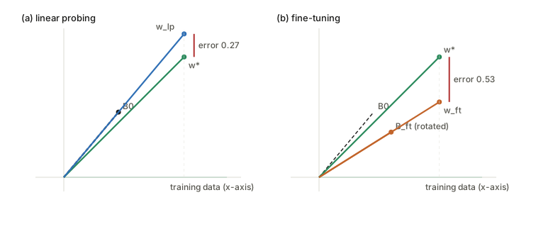
The 2-D toy of the paper’s Figure 2, run as an actual gradient flow (k=1, d=2; B_0 at 50^\circ, truth at 45^\circ, head started at 0.5). The vertical coordinate of the feature never moves; only its horizontal one does.
Result 4: Theorem 3.5, LP beats FT OOD for good features
LP error. With A_0=XB_0^\top (tall, n\ge m>k) the LP loss \lVert A_0v-Y\rVert^2 is strongly convex, with unique minimiser v_{\rm lp}^\infty=(A_0^\top A_0)^{-1}A_0^\top Y. Since Y=XB_\star^\top v_\star,
v_{\rm lp}^\infty-v_\star=(A_0^\top A_0)^{-1}A_0^\top X(B_\star-B_0)^\top v_\star, \qquad \lVert v_{\rm lp}^\infty-v_\star\rVert\le\frac{\lVert X\rVert\,\epsilon\,\lVert v_\star\rVert}{\sigma_{\min}(A_0)},
and \sigma_{\min}(A_0)\ge\sigma_{\min}(Z)\cos\theta_{\max}(R_0,S), where X=ZF^\top (F an orthonormal basis of S). Adding the feature error \lVert(B_\star-B_0)^\top v_\star\rVert\le\epsilon\lVert v_\star\rVert gives Lemma A.14: \sqrt{L_{\rm ood}(v_{\rm lp}^\infty,B_0)}\le c_\delta\,\epsilon\lVert w_\star\rVert/\cos\theta_{\max}(S,R). (This is my reconstruction of the displayed lemma; the paper hides the Z-dependent factors in a constant c_\delta, and for Gaussian P_z with n\ge5m gives O(\log(n/\delta))\,\epsilon\lVert w_\star\rVert/\cos^2\theta_{\max}.) LP error is first order in \epsilon, i.e. its squared loss is O(\epsilon^2).
FT error. Theorem 3.3 with Lemma A.12 (a Gaussian head has \varphi^2\ge c_\delta>0 with probability 1-\delta/2): \inf_t\sqrt{L_{\rm ood}}\ge c'_\delta-\epsilon. This tends to a positive constant as \epsilon\to0.
Dividing: the ratio L_{\rm ood}(\mathrm{LP})/\inf_tL_{\rm ood}(\mathrm{FT})\to0 in probability as B_0\to B_\star (Theorem 3.5 / A.8). A random S makes both non-degeneracy conditions hold almost surely (Lemma A.16).
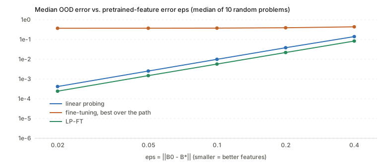
Medians over 10 random problems per point.
| \epsilon | LP | FT, best over t | LP-FT, end | LP / FT |
|---|---|---|---|---|
| 0.40 | 0.1407 | 0.4397 | 0.0837 | 0.291 |
| 0.20 | 0.0386 | 0.3937 | 0.0221 | 0.094 |
| 0.10 | 0.0100 | 0.3788 | 0.0057 | 0.027 |
| 0.05 | 0.0026 | 0.3734 | 0.0015 | 0.0070 |
| 0.02 | 0.0004 | 0.3708 | 0.0002 | 0.0012 |
LP falls like \epsilon^2; FT’s best iterate stalls at about 0.37 however good the features get. That plateau is exactly what “the bound does not vanish as \epsilon\to0” says.
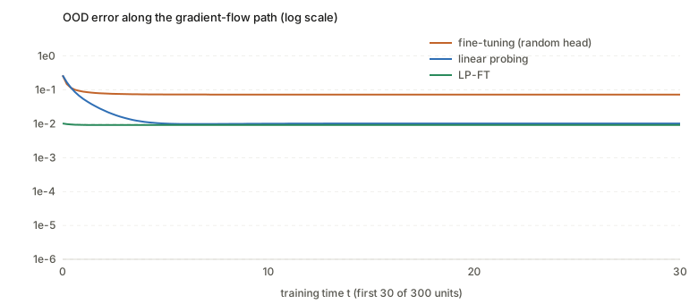
One instance, \epsilon=0.1. FT’s OOD error is lowest at its end, so early stopping would not have helped. The paper’s Section 4.3 reports the same for real networks (linear probing 67.1% against 61.3% for FT even when FT is early-stopped on OOD data).
Result 5: Proposition 3.6, FT wins ID
If w_\star\notin R_0 (the pretrained features are imperfect) and \cos\theta_{\max}(S,R_{\rm aug})\ne0, with R_{\rm aug}=\operatorname{span}(R_0\cup\{w_\star\}):
- FT reaches zero training loss. For a two-layer linear network every local minimum is global (Laurent & von Brecht 2018), and (v_\star,B_\star) gets zero loss, so if the flow converges to a local minimum it fits the training set exactly. n\ge m points span S almost surely, so linear-in-x predictors that agree on the training set agree on all of S: L_{\rm id}=0.
- LP does not. LP’s predictor is x\mapsto v^\top B_0x, a function in the k-dimensional space spanned by the rows of B_0 restricted to S. It matches w_\star on S exactly only if F^\top w_\star\in\operatorname{Range}(F^\top E_0) (Lemma A.18). Lemma A.17 shows that when F^\top E_{\rm aug} has full rank k+1 (which is what \cos\theta_{\max}(S,R_{\rm aug})>0 says, using m>k) this membership fails. So L_{\rm id}(\mathrm{LP})>0.
Numerically: ID error at the end is 8.6\times10^{-30} for FT and 1.2\times10^{-3} for LP (at \epsilon=0.1).
Result 6: Proposition 3.7, why starting from the LP head can help
Suppose B_0=UB_\star (perfect features up to rotation). Prop. A.20: LP then recovers v_{\rm lp}^\infty=Uv_\star because A_0^\top A_0 is invertible and v=Uv_\star has zero loss. Now start FT at (v_{\rm lp}^\infty,B_0). The training residual is r=XB_0^\top v-Y=0, so
\nabla_v\widehat L=2B_0X^\top r=0,\qquad\nabla_B\widehat L=2\,v\,r^\top X=0 .
Nothing moves, so L_{\rm ood}=0 for all t (LP-FT). With a random head v_0\sim N(0,\sigma^2I) the same setting has \varphi\ne0 almost surely, so Theorem 3.3 with \epsilon=0 gives L_{\rm ood}>0 for all t (FT). Checked (\epsilon=0): LP-FT’s OOD error stays at \sim10^{-32}; FT from a random head never goes below 2.13 (it starts at 3.47).
This is a first cut, the authors say. With perfect features LP alone already gets zero OOD error, so the proposition shows that LP-FT does not damage the features but not that it improves on LP. For imperfect features there is no proof (“no closed form for the iterates, we were not able to show an upper bound”). The simulation does show it empirically (table above, LP-FT column below LP at every \epsilon, and the feature extractor changes by 0.033 against 0.244 for FT).
Experiments, in one table
ID/OOD accuracy averaged over datasets, CLIP and MoCo-v2 features (the paper’s Tables 1–2; ResNet-50, plus CLIP ViT-B/16 on ImageNet):
| ID | OOD | |
|---|---|---|
| FT | 85.1 | 59.3 |
| LP | 82.9 | 66.2 |
| LP-FT | 85.7 | 68.9 |
Checks of the theory’s mechanism (Section 4.3, Living-17): distance moved by features after FT is 0.0188 for ID inputs and 0.0167 for OOD inputs (larger on ID), and LP-FT moves both by about 0.001. FT beats LP OOD only for worse features (MoCo-v1) or a tiny shift (CIFAR-10 → CIFAR-10.1: 92.3 against 82.7), exactly where the theory’s hypotheses fail.
What the toy figure actually says
The paper’s Figure 2 is a cartoon, and the numbers depend on the
geometry. Running the exact gradient flow for the 2-D problem gives the
vertical-axis (OOD) error for several tilts of B_0 and several initial heads (true head size
\lVert v_\star\rVert=2;
part5_toy_2d):
| tilt of B_0 (truth: 45°) | LP | FT, v_0=0 | v_0=0.5 | v_0=1 | v_0=2 | v_0=3 |
|---|---|---|---|---|---|---|
| 46° | 0.050 | 0.628 | 0.593 | 0.477 | 0.027 | 0.713 |
| 50° | 0.271 | 0.567 | 0.529 | 0.404 | 0.133 | 0.860 |
| 55° | 0.605 | 0.495 | 0.454 | 0.319 | 0.255 | 1.029 |
| 60° | 1.035 | 0.429 | 0.384 | 0.240 | 0.366 | 1.180 |
Three things to read off: LP’s error grows with the tilt (it overshoots, since it matches only the horizontal coordinate); FT’s depends on the head and is smallest when \lVert v_0\rVert is near the true 2 (\varphi\approx0: the bound vanishes); and for tilts of 55° and more FT wins. The theorem is about the small-\epsilon regime, and the toy shows that outside it the ordering can flip.
Questions and doubts
- What are the constants? Theorem 3.3 is stated with O(\cdot) hiding a universal constant that the proof does not make explicit, and the bound has a -\epsilon term. So it is vacuous unless \epsilon is below a threshold that depends on \varphi,c,k,\lVert w_\star\rVert, and the authors do not say how small. The simulation is consistent with the shape (FT stalls at ≈0.37 for \epsilon\le0.4), but nothing in the paper says where real feature extractors sit relative to the threshold. The authors note the -\epsilon is there because “the errors can cancel” and hope future work captures why they usually will not.
- Is the mechanism “unchanged outside the span” really operating in deep nets? For ImageNet, n=1.28M exceeds the input dimension (\approx150k), so the inputs span all of \mathbb R^d and S^\perp=\{0\}: Lemma A.3 gives nothing literally. The mechanism has to survive in a softer form (feature change that is larger on ID than on OOD, which the Living-17 numbers support), and the authors’ own footnote suggests the NTK view, where d is the number of weights and exceeds n. That extension is left open, so the theory explains the direction of the effect but does not predict its size.
- Lemma A.4 is a gradient-flow, no-weight-decay fact. Real fine-tuning uses Adam or SGD with momentum, a learning-rate schedule, weight decay, normalisation layers. Weight decay breaks balancedness immediately; Adam rescales each coordinate. The claim “never passes through a good point” is for the exact flow only. I did not test any of these variants.
- “Early stopping cannot fix FT” is partly mechanical. The bound holds at every t including t=0, where the random head is bad. The informative content is that the minimum over the path stays at the floor (0.379 median at s=0 versus 0.0057 for LP-FT), not that early stopping fails in some further sense.
- Where does the LP-FT guarantee for imperfect features come from? Only from experiments (and my simulation, which shows FT-from-LP-head ending below LP’s OOD error at every \epsilon I tried). Intuitively the head that LP finds is far from v_\star by O(\epsilon), so \varphi=O(\epsilon) and the extractor moves by O(\epsilon). A clean statement would be an upper bound of that form, which the paper says it could not prove.
- Linear probing here is the exact least-squares solution. In the experiments LP is \ell_2-regularised logistic regression, where the head norm is capped; the analysis (and Lemma A.14) is for the unregularised convex problem. The link needs a continuity argument that is not written.
- A slip in Step 2A. (A.49) writes the rearranged balancedness identity with v_\star v_\star^\top where the identity gives v_{\rm ft}v_{\rm ft}^\top. The correct bound is \lVert B_{\rm ft}\rVert_F^2\le\lVert B_0\rVert_F^2+\lVert v_{\rm ft}\rVert^2 with \lVert v_{\rm ft}\rVert\le\lVert v_\star\rVert+(\Delta+\epsilon\lVert v_\star\rVert)/c from Step 1. This adds a term of the same order as the others, so the form of the final bound should survive, but the constants in (A.85)–(A.91) are not exactly as written.
- Typos in the appendix (harmless): (A.6) writes \cos\theta_r\le0 where \ge0 is meant; Lemma A.5’s proof swaps the dimension labels of E and F; Lemma A.7 prints “\le\sigma_{\min}” for “\ge\sigma_{\min}”; Step 1 cites “Proposition A.3” for Lemma A.3. The big-O convention (constants may change between lines) makes line-by-line verification of (A.85)–(A.91) impossible without the authors’ constants.
- What about the minimum principal angle? The authors conjecture the bound holds with \cos\theta_{\min}(R_0,S^\perp) (error in every direction outside S). Careful: the error functional on S^\perp is x\mapsto(B_0^\top v_{\rm ft}-w_\star)^\top x, a single linear functional, so it vanishes on a hyperplane of S^\perp. The conjecture can only mean a worst-case statement over directions, not “all directions”.
Takeaways
- Fine-tuning does not just improve features; it changes them unevenly. Directions that the labelled data does not touch keep their pretrained values, and the head learns to expect the changed ones.
- Two exact facts do the work: the gradient on the extractor lives in the span of the training inputs, and vv^\top-BB^\top is conserved. Both survive a change of loss function.
- The damage is controlled by the head’s initial misalignment \varphi^2=|(v_0^\top v_\star)^2-\lVert v_\star\rVert^4| (my simulation: best OOD error 0.379 → 0.0057 as the head goes from random to the LP solution) and it does not vanish as the pretrained features improve (FT stalls near 0.37 while LP falls like \epsilon^2).
- LP-FT is the cheapest way to get \varphi small: one convex fit, then the usual fine-tune. It is a heuristic with a proof only at perfect features.
- A tilted pretrained feature with a large distribution shift is the regime where LP wins. For a badly tilted extractor, or a small shift, FT can win OOD. The paper’s experiments show both cases.
Notes written 2026-10-14.