A Statistical Theory of Overfitting for Imbalanced Classification
Links
- arXiv:2502.11323: the preprint (the ICLR 2026 camera-ready is the version read here). Code: jlyu55/Imbalanced_Classification.
- Interactive companion: six widgets. (1) Training vs test logits for any (\pi,\lVert\mu\rVert,\delta,\tau), solved from the paper’s equations, with a real hard-margin SVM you can train in the browser on top. (2) The separability threshold \delta^*(0). (3) Errors against \tau and \pi. (4) The three high-imbalance phases. (5) The proximal map of the non-separable case. (6) The limiting reliability curve.
- Runnable
checks:
asymptotics.pysolves the limiting equations and checks the algebra.svm_simulation.pytrains exact hard-margin SVMs (dual SMO) and compares them with the limits.make_figures.pydraws the three figures below. Every number in these notes is printed by one of them.make verifyruns all three. - Optimal transport: the pushforward T_\sharp and the Wasserstein distance W_2 used to state the convergence of logit distributions.
- The Price of Robustness: another paper in this collection that reads overfitting through margins.
In one paragraph
Train a linear classifier f(x)=\langle x,\beta\rangle+\beta_0 on n points in d dimensions, with n and d of the same order. The paper asks what the logits f(x_i) look like on the training set compared with a fresh test set. It works in the simplest model where the question can be answered exactly: two Gaussian classes x\mid y\sim\mathcal N(y\mu,I_d), a minority fraction \pi<\tfrac12, and the max-margin classifier (the hard-margin SVM, which is also where logistic regression’s gradient descent ends up on separable data). The answer (Theorem 2.1) is clean. On test data the signed logit y f(x) is a Gaussian \mathcal N(\rho^*\lVert\mu\rVert+y\beta_0^*,1). On training data it is the same Gaussian with everything below the margin \kappa^* moved onto \kappa^*: \max\{\kappa^*,\ \text{that Gaussian}\}. The three numbers (\rho^*,\beta_0^*,\kappa^*) solve a small variational problem. Its core is a budget: the d “free” directions can move the n training logits by a mean square of at most 1/\delta, where \delta=n/d. The fit spends that budget on lifting every training point up to the margin, which is exactly a truncation. The intercept comes out negative, so the minority’s test Gaussian sits closer to the boundary. Its truncated mass is therefore larger (61% vs 18% in the paper’s Figure 1 setting), and so is its test error (25% vs 3%). A per-point identity makes this sharp: the average lift of a minority point is exactly (1-\pi)/\pi times that of a majority point. The rest of the paper follows from the same equations. It gives the optimal margin-rebalancing ratio \tau^{\rm opt} in closed form and three phases when \pi\to0 with d. It also gives a limiting calibration error, and it covers the non-separable case, where the truncation becomes a proximal shrinkage. I checked everything numerically, and the theory matches finite SVMs closely. Two things need care. First, in the paper’s own calibration experiments \tau^{\rm opt} is negative, outside the proven range. Second, the growth of miscalibration with imbalance is almost entirely the prior log-odds that rebalancing deliberately throws away. It is not overfitting.
Background, from the ground up
Logits, margins, and why “training accuracy 100%” hides the interesting part
A linear classifier predicts \hat y=+1 when f(x)>0. The number f(x) is the logit, and y f(x) (the logit signed by the true label) is positive exactly when the prediction is right. The size of y f(x) says by how much. With \lVert\beta\rVert=1 it is literally the signed distance from x to the decision hyperplane. The margin of a classifier on the training set is the smallest of these, \hat\kappa_n=\min_i y_i f(x_i) (Definition 2.1). The max-margin classifier maximises it:
\max_{\beta,\beta_0,\kappa}\ \kappa\quad\text{s.t.}\quad y_i(\langle x_i,\beta\rangle+\beta_0)\ge\kappa\ \ \forall i,\qquad \lVert\beta\rVert_2\le1. \qquad\text{(Eq 2b)}
If the training data are linearly separable, \hat\kappa_n>0 and training accuracy is 100%. In high dimensions that is typical, and the test accuracy is still imperfect. Accuracy compresses each logit to one bit, right or wrong. The paper keeps the whole histogram of logits, on training points and on test points, and reads overfitting off the difference.
Why the SVM and not logistic regression? On separable data the logistic loss has no finite minimiser: scaling \beta up always lowers it. Gradient descent then runs off to infinity, but its direction \beta^{(t)}/\lVert\beta^{(t)}\rVert converges to the max-margin direction (Soudry et al. 2018; App C.2 extends this to include the intercept, Proposition C.2). So the SVM is what a linear probe trained to convergence actually is, up to scale.
Proportional asymptotics
Classical statistics lets n\to\infty with d fixed. Then the fitted \hat\beta converges to the truth, and training and test logits look alike. Here instead n,d\to\infty with n/d\to\delta\in(0,\infty), the aspect ratio. A small \delta means few samples per dimension. In this limit random quantities like the cosine \hat\rho=\langle\hat\beta/\lVert\hat\beta\rVert,\mu/\lVert\mu\rVert\rangle do not go to 1. They go to a deterministic number \rho^*<1 that depends on (\pi,\lVert\mu\rVert,\delta). The whole paper computes such numbers.
Notation for distributions, in plain words
The paper states its results about distributions. The notation is measure-theoretic, but each piece has a plain meaning:
- \mathrm{Law}(Z) is just “the distribution of the random variable Z”. For example, \mathrm{Law}(Y,\,Y\max\{\kappa,G\}) is the joint distribution of the pair you get by drawing a label Y, drawing G\sim\mathcal N(0,1), and computing Y\max\{\kappa,G\}.
- \delta_a (a Dirac mass) is the distribution that puts all its probability on the single point a. So \frac1n\sum_i\delta_{(y_i,f(x_i))} puts mass 1/n on each training pair. It is the training histogram, written as a distribution (Eq 3). This is the ELD, the empirical logit distribution. The TLD is \mathrm{Law}(y_{\rm test},f(x_{\rm test})) for a fresh point.
- W_2(P,Q), the 2-Wasserstein distance, is the smallest root-mean-square distance you have to move the mass of P to turn it into Q. For two 1-D samples of equal size, sort both and pair them up; W_2 is the RMS gap between the paired values. “W_2(\hat\nu_n,\nu_*)\to0” says the training histogram, including its tails, approaches the limit. The OT page has pictures.
- \xrightarrow{w} (weak convergence) says the probabilities of intervals converge. It is weaker than W_2 and is what one gets for the test logit of a single fresh point.
- \xi\in L^2: in Eq 5 the unknown is a whole random variable \xi with finite second moment. Read it as “a rule assigning a number \xi to every possible draw of (Y,G)”. The optimiser gets to choose that rule, subject only to \mathbb E[\xi^2]\le1/\delta. It turns out to be a deterministic function of (Y,G).
- T_\sharp\mu (pushforward): the distribution of T(X) when X\sim\mu. In Proposition D.2, T_\sharp L^{\rm test}_*=L_* says “apply T(x)=\max\{\kappa^*,x\} to a test logit and you get something distributed like a training logit”.
Two Gaussian integrals that do all the work
With G\sim\mathcal N(0,1), \Phi its CDF and \varphi its density, define
g_1(t)=\mathbb E[(G+t)_+]=t\,\Phi(t)+\varphi(t),\qquad g_2(t)=\mathbb E[(G+t)_+^2]=(t^2+1)\Phi(t)+t\,\varphi(t). \qquad\text{(Eq 75)}
Here a_+=\max\{a,0\}. If a Gaussian
sits t below some level, g_1(t) is the average amount by which it
falls short, counting only the points that fall short. g_2(t) is the mean squared shortfall. Both
are strictly increasing. asymptotics.py §1 checks the
closed forms against Monte Carlo: for example g_1(0)=1/\sqrt{2\pi}=0.3989 and g_2(0)=\tfrac12.
The spine of the argument
- Decompose \beta into signal and free directions. Write \beta=\rho\,\mu/\lVert\mu\rVert+\sqrt{1-\rho^2}\,\theta with \theta\perp\mu. The honest part of a training logit is y_i f(x_i)\approx \rho\lVert\mu\rVert+G_i+y_i\beta_0. The \theta part lives in d-1 noise directions that the classifier can bend towards individual training points.
- Gordon’s comparison removes the random matrix. The max-margin problem is a min–max of a bilinear form in a Gaussian matrix. The convex Gaussian min–max theorem (CGMT) replaces it by a problem with two random vectors, which collapses to three scalars (\rho,r,\beta_0).
- The collapsed problem is a budget. Data are separable at margin \kappa iff \delta\,\mathbb E[(s(Y)\kappa-X)_+^2]\le1-\rho^2 for some (\rho,\beta_0), where X=\rho\lVert\mu\rVert+G+Y\beta_0. In words: the mean squared lift needed to bring every point up to the margin must fit inside what the free directions can supply. This gives the separability threshold \delta^*(0) and the limit margin \kappa^*.
- Truncation is the cheapest way to spend the budget. The least-energy lift raises points below \kappa exactly to \kappa and leaves the rest alone. A pointwise Pythagorean inequality turns this into W_2 convergence of the ELD to \max\{\kappa^*,X\}.
- First-order conditions give everything else in closed form. \rho^* solves one scalar equation. \beta_0^*<0 follows at once. \tau moves only the intercept. \tau^{\rm opt}, the errors and the calibration limits are all explicit.
Setup and notation
| Symbol | Meaning |
|---|---|
| \pi=\mathbb P(y=+1)<\tfrac12 | minority fraction; the minority is labelled +1 |
| x\mid y\sim\mathcal N(y\mu,I_d) | the 2-GMM (Eq 1); \lVert\mu\rVert is the signal strength, class centres \pm\mu |
| \delta=\lim n/d | aspect ratio; small \delta = many dimensions per sample |
| f(x)=\langle x,\beta\rangle+\beta_0, \lVert\beta\rVert=1 | the classifier; y f(x) is the signed distance to the boundary |
| \hat\rho=\langle\hat\beta,\mu/\lVert\mu\rVert\rangle | cosine between the learned and the Bayes direction |
| \tau>0, s(y)=\tau if y=+1, else 1 | margin ratio: the minority must clear \tau\kappa, the majority \kappa (Eq 7) |
| (Y,G)\sim P_y\times\mathcal N(0,1) | a generic label and a standard Gaussian in the limit problems |
| X=\rho\lVert\mu\rVert+G+Y\beta_0 | the “honest” signed logit: what y f(x) is on a test point |
| \xi | the overfitting variable: extra lift of a training logit from the free directions |
| \mathrm{Err}_\pm | minority / majority test error (Eq 4); \mathrm{Err}_b their average |
| g_1,g_2 | \mathbb E(G+t)_+, \mathbb E(G+t)_+^2 (Eq 75) |
| \delta^*(\kappa) | largest \delta at which margin \kappa is still attainable (Eq 28) |
Theorem 2.1: the logits, the variational problem, and what it means
The statement
For \delta<\delta_c the data are separable with high probability. The trained parameters converge, (\hat\rho,\hat\beta_0,\hat\kappa)\to(\rho^*,\beta_0^*,\kappa^*), where these solve
\max_{\rho\in[-1,1],\,\beta_0,\,\kappa>0,\,\xi\in L^2}\ \kappa\quad\text{s.t.}\quad \underbrace{\rho\lVert\mu\rVert+G+Y\beta_0}_{X}+\sqrt{1-\rho^2}\,\xi\ \ge\ \kappa\ \ \text{a.s.},\qquad \mathbb E[\xi^2]\le\frac1\delta. \qquad\text{(Eq 5)}
The errors converge to \mathrm{Err}_+\to\Phi(-\rho^*\lVert\mu\rVert-\beta_0^*) and \mathrm{Err}_-\to\Phi(-\rho^*\lVert\mu\rVert+\beta_0^*). The logit distributions converge to
\nu_*^{\rm train}=\mathrm{Law}\big(Y,\;Y\max\{\kappa^*,\,X^*\}\big),\qquad \nu_*^{\rm test}=\mathrm{Law}\big(Y,\;Y X^*\big),\qquad X^*=\rho^*\lVert\mu\rVert+G+Y\beta_0^*.
(The general version, Theorem D.1, has s(Y)\kappa in place of \kappa for the rebalanced SVM.)
Reading Eq 5 term by term
- Where X comes from. Take a fresh point x=y\mu+z with z\sim\mathcal N(0,I_d) independent of \hat\beta. Then y f(x)=\langle\mu,\beta\rangle+y\langle z,\beta\rangle+y\beta_0. The first term is \rho\lVert\mu\rVert. The second is \mathcal N(0,1), because \lVert\beta\rVert=1 and z is isotropic (the sign y does not matter). So a test logit is exactly X. This one line is the TLD, and it gives the test errors: the minority is wrong when \rho\lVert\mu\rVert+G+\beta_0\le0, which has probability \Phi(-\rho\lVert\mu\rVert-\beta_0).
- Where \xi comes from. On a training point, z_i is not independent of \hat\beta, because \hat\beta was chosen after seeing it. The component \sqrt{1-\rho^2}\,\theta in the d-1 directions orthogonal to \mu carries no signal. What it can do is correlate with the particular noise vectors z_i and push chosen training logits up. \sqrt{1-\rho^2}\,\xi is that push.
- Why \mathbb E[\xi^2]\le1/\delta. A heuristic: to raise training point j by t_j, add t_j z_j/d to \theta. Since \langle z_j,z_j\rangle\approx d, this lifts point j by t_j. It moves each other point by only O(t_j/\sqrt d) and adds t_j^2/d to \lVert\theta\rVert^2. Doing it for all n points costs \sum_j t_j^2/d=\delta\cdot\overline{t^2} of squared norm, where \overline{t^2} is the mean squared lift. A unit budget of norm therefore buys \overline{t^2}\lesssim1/\delta. With few samples per dimension (small \delta) the budget is large and overfitting is severe; as \delta\to\infty it vanishes. (The cross-talk between points is of the same order, and handling it exactly is what Gordon’s theorem does. The heuristic gets the scaling right, not the constant.)
- What is being traded. A larger \rho puts more weight on the signal, raising every X by \rho\lVert\mu\rVert. But it leaves less norm \sqrt{1-\rho^2} for the free directions, so each unit of \xi lifts less. The optimum balances the two.
Solving the inner problem: the lift is a truncation (Eq 6)
Fix (\rho,\beta_0,\kappa). Which \xi satisfies the constraint with the least energy \mathbb E\xi^2? The constraint is pointwise: \sqrt{1-\rho^2}\,\xi\ge\kappa-X. Where X\ge\kappa it asks nothing, so \xi=0 is cheapest. Where X<\kappa it asks for at least \kappa-X, and anything more wastes energy. So
\sqrt{1-\rho^2}\,\xi^*=(\kappa-X)_+,\qquad X+\sqrt{1-\rho^2}\,\xi^*=\max\{\kappa,X\}. \qquad\text{(Eqs 6, 32)}
That is the whole reason the training logits are truncated. It is the least-energy way to put every training point on the correct side of the margin. The appendix proves it with KKT conditions for the infinite-dimensional problem (proof of Theorem D.1(b)); the pointwise argument above is the same thing. Plugging \xi^* back in, the budget constraint becomes
\mathbb E\big[(s(Y)\kappa-X)_+^2\big]\ \le\ \frac{1-\rho^2}{\delta} \iff H_\kappa(\rho,\beta_0):=\frac{1-\rho^2}{\mathbb E[(s(Y)\kappa-\rho\lVert\mu\rVert-G-Y\beta_0)_+^2]}\ \ge\ \delta, \qquad\text{(Eqs 28, 33)}
and the limit problem is “maximise \kappa subject to H_\kappa(\rho,\beta_0)\ge\delta”. Write \delta^*(\kappa)=\max_{\rho,\beta_0}H_\kappa. Margin \kappa is attainable iff \delta\le\delta^*(\kappa). The data are separable iff \delta<\delta^*(0) (Theorem D.1(a)), and \kappa^* is where \delta^*(\kappa^*)=\delta.
Sanity check: Cover’s theorem. With no signal (\mu=0) and balanced classes, take \rho=\beta_0=0: \delta^*(0)=1/g_2(0)=2. That is Cover’s
classical result that n random points
in general position in \mathbb R^d are
separable with random labels up to n\approx2d. asymptotics.py §2
recovers 2.0000. Other values: with \mu=0 and \pi=0.15 the threshold is 3.10. The intercept
alone separates more when the labels are unbalanced. It is 3.70 at \lVert\mu\rVert=1,\pi=\tfrac12, and 18.0 at
the paper’s Figure 1 setting (\lVert\mu\rVert=1.75,\pi=0.15), so \delta=2.5 there is deep in the separable
regime. Widget 2 of the interactive page plots \delta^*(0) against \pi.
The closed-form solution (Lemma E.9)
The constraint F(\rho,\beta_0,\kappa)=\delta\,\mathbb E[(s\kappa-X)_+^2]-(1-\rho^2)\le0 is convex. At the optimal \kappa^* the feasible set in (\rho,\beta_0) shrinks to one point. That point minimises F, with minimum value 0. Split the expectation by class, with m=\lVert\mu\rVert and the two gaps t_+=\tau\kappa-\rho m-\beta_0 (minority) and t_-=\kappa-\rho m+\beta_0 (majority):
F=\pi\delta\,g_2(t_+)+(1-\pi)\delta\,g_2(t_-)+\rho^2-1,\qquad g_2'=2g_1.
The two stationarity conditions and F=0 give
\partial_{\beta_0}F=0:\ \ \pi\,g_1(t_+)=(1-\pi)\,g_1(t_-),\qquad \partial_\rho F=0\ \text{(with the first)}:\ \ g_1(t_+)=\frac{\rho}{2\pi m\delta},\ \ g_1(t_-)=\frac{\rho}{2(1-\pi)m\delta}, \qquad\text{(Eqs 77, 79)}
\pi\delta\,g\Big(\tfrac{\rho}{2\pi m\delta}\Big)+(1-\pi)\delta\,g\Big(\tfrac{\rho}{2(1-\pi)m\delta}\Big)=1-\rho^2,\qquad g=g_2\circ g_1^{-1}. \qquad\text{(Eq 76a)}
Eq 76a is one equation in \rho
alone. Its left side rises from 0 and its right side falls to 0, so it
has exactly one root \rho^*\in(0,1). It
does not involve \tau. Then t_\pm=g_1^{-1}(\cdot) give \kappa^* and \beta_0^* by two linear equations (76b, 76c).
asymptotics.py §3 solves this at Figure 1’s setting (\lVert\mu\rVert=1.75, \pi=0.15, \delta=2.5):
| \rho^* | \beta_0^* | \kappa^* | \mathrm{Err}_+ | \mathrm{Err}_- | \mathrm{Err}_b | |
|---|---|---|---|---|---|---|
| limit | 0.7235 | −0.5960 | 0.9447 | 25.1% | 3.1% | 14.1% |
| SVM, n=2000, d=800 (3 draws) | 0.735 ± 0.005 | −0.600 ± 0.039 | 0.960 ± 0.020 | 24.7% | 3.0% |
For scale: the Bayes classifier has 10.5% and 1.2%, and the best balanced error with the true direction is \Phi(-\lVert\mu\rVert)=4.0\%. The budget is spent exactly: \mathbb E[(s\kappa^*-X^*)_+^2]=0.19064=(1-\rho^{*2})/\delta.
Why the minority suffers: two one-line consequences
The per-point push. g_1(t_\pm) is the average lift a point of each class receives (on the event that it is lifted). The \beta_0 condition says
\pi\,g_1(t_+)=(1-\pi)\,g_1(t_-)\qquad\Longleftrightarrow\qquad \frac{g_1(t_+)}{g_1(t_-)}=\frac{1-\pi}{\pi}.
Each class receives the same total push. The intercept is chosen so that neither class’s margin constraint is binding harder than the other’s. The minority has \pi/(1-\pi) times fewer points to share it, so each minority point is pushed (1-\pi)/\pi times further. At Figure 1: 0.551 vs 0.097, a ratio of 5.667 = 0.85/0.15 (§4). This is the paper’s “common overfitting budget” made exact.
The intercept is negative. Subtract 76c from 76b at \tau=1:
2\beta_0^*=g_1^{-1}\Big(\tfrac{\rho^*}{2(1-\pi)m\delta}\Big)-g_1^{-1}\Big(\tfrac{\rho^*}{2\pi m\delta}\Big)<0\qquad(\pi<\tfrac12),
because g_1^{-1} is increasing. (At Figure 1: -1.192.) So the minority’s test centre \rho^*m+\beta_0^*=0.67 sits much closer to the boundary than the majority’s \rho^*m-\beta_0^*=1.86. The same margin \kappa^* then truncates 60.8% of the minority and 17.9% of the majority, and the mass below 0 (the test error) is 25.1% against 3.1%.
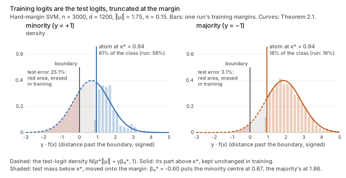
The simulated ELD matches the limit well at this modest size.
svm_simulation.py §2 gives these deciles of y_i f(x_i):
| quantile | 0.1 | 0.3 | 0.5 | 0.7 | 0.9 |
|---|---|---|---|---|---|
| minority, SVM | 0.958 | 0.958 | 0.958 | 1.094 | 1.896 |
| minority, limit | 0.945 | 0.945 | 0.945 | 1.195 | 1.956 |
| majority, SVM | 0.958 | 1.424 | 1.912 | 2.427 | 3.231 |
| majority, limit | 0.945 | 1.339 | 1.863 | 2.387 | 3.148 |
The atom is the support vectors. The point mass at \kappa^* consists of the training points exactly on the margin. In the SVM these are the support vectors. The limit predicts n[\pi\Phi(\kappa^*-\rho^*m-\beta_0^*)+(1-\pi)\Phi(\kappa^*-\rho^*m+\beta_0^*)]=0.244\,n of them, which is 0.61 per dimension. That has to be at most 1: a hard-margin SVM in general position has at most d+1 support vectors. The simulation has 474 against a predicted 488, with d+1=801. The paper does not make this connection, but it is a nice consistency check on the theory.
The optimal-transport remark (Proposition D.2)
T(x)=\max\{\kappa^*,x\} is the optimal transport map from L^{\rm test}_* to L_* for any strictly convex cost. The proof is one line. In 1-D the optimal map between two distributions is always the monotone rearrangement F_\nu^{-}\circ F_\mu (quantile of the target composed with CDF of the source). Here that composition equals \max\{\kappa^*,x\}. So the statement is true, but it holds for any monotone map between 1-D laws. It adds a name to Eq 6 rather than new information. The more useful fact, used in the proof below, is a Pythagorean inequality.
The proof of Theorem 2.1 (Appendix E), step by step
Step 0: separability as the zero set of a random min–max
Margin \kappa is achievable iff the vector of shortfalls (\kappa s_y-y\odot X\beta-\beta_0 y)_+ can be made zero. Define
\xi_{n,\kappa}=\min_{\lVert\beta\rVert\le1,\ \beta_0}\ \tfrac1{\sqrt d}\big\lVert(\kappa s_y-y\odot X\beta-\beta_0y)_+\big\rVert_2 =\min_{\beta,\beta_0}\ \max_{\lVert\lambda\rVert\le1,\ \lambda\odot y\ge0}\ \tfrac1{\sqrt d}\lambda^\top(\kappa s_y\odot y-X\beta-\beta_0\mathbf 1). \qquad\text{(Eq 47)}
The second form uses \lVert a_+\rVert_2=\max_{\lVert\lambda\rVert\le1,\lambda\ge0}\lambda^\top a (the best unit vector to align with a is a_+/\lVert a_+\rVert). So \xi_{n,\kappa}=0 iff margin \kappa is attainable, and \hat\kappa_n=\sup\{\kappa:\xi_{n,\kappa}=0\}. Only the sign of \xi_{n,\kappa} matters. The magnitude never enters, and that freedom is used in Step 4.
Step 1: the intercept stays bounded (Lemma E.1)
Gordon’s theorem needs compact constraint sets, and \beta_0 is unconstrained. On the separable event, pick one minority and one majority point. The constraints bound |\beta_0| by (\tau+1)\kappa+2\lVert\mu\rVert plus the largest projections of the noise. Averaging over each class and using \lVert Z_\pm\rVert_{\rm op}\approx\sqrt{n_\pm}+\sqrt d gives a constant bound B_0 with high probability. So restricting to |\beta_0|\le B changes nothing asymptotically.
Step 2: Gordon’s comparison (Lemma E.2)
Write x_i=y_i\mu+z_i and split \beta=\rho\,\mu/\lVert\mu\rVert+\theta with \theta\perp\mu, \lVert\theta\rVert\le\sqrt{1-\rho^2}. The objective becomes \lambda^\top\mathbf G\theta+(\text{terms in }\rho,\beta_0,y,u), where \mathbf G\in\mathbb R^{n\times(d-1)} has i.i.d. \mathcal N(0,1) entries (the noise orthogonal to \mu) and u_i=\langle z_i,\mu\rangle/\lVert\mu\rVert. The random matrix appears only in the bilinear term. The CGMT (Lemma J.1) says that
\min_\theta\max_\lambda\ \lambda^\top\mathbf G\theta+\psi(\theta,\lambda) \quad\text{and}\quad \min_\theta\max_\lambda\ \lVert\lambda\rVert\,g^\top\theta+\lVert\theta\rVert\,h^\top\lambda+\psi(\theta,\lambda), \qquad g\sim\mathcal N(0,I_{d-1}),\ h\sim\mathcal N(0,I_n),
have comparable distributions. The first is below any level at most twice as often as the second. If the sets are convex and \psi is convex–concave, the same holds for “above”, which is what pins down the value. Why is this plausible? For fixed (\theta,\lambda) both \lambda^\top\mathbf G\theta and \lVert\lambda\rVert g^\top\theta+\lVert\theta\rVert h^\top\lambda are centred Gaussians. Gordon’s inequality compares the min–max of two Gaussian processes whose covariances are ordered in the right way. The payoff: an n\times d random matrix is replaced by two random vectors, and those can be handled one coordinate at a time.
Step 3: collapse to three scalars (Lemma E.3)
Two elementary maximisations finish the reduction. Over \lambda: \max_{\lVert\lambda\rVert\le1,\lambda\ge0}(a\lVert\lambda\rVert+\lambda^\top b)=(a+\lVert b_+\rVert)_+. Over the direction of \theta at fixed length r: \min g^\top\theta=-r\lVert g\rVert, taking \theta along -g. With \lVert g\rVert/\sqrt d\to1, n/d\to\delta and a uniform law of large numbers on the compact set of (\rho,r,\beta_0),
\xi_{n,\kappa}\ \xrightarrow{p}\ \Big(\min_{\rho^2+r^2\le1,\,r\ge0,\,|\beta_0|\le B}\ -r+\sqrt\delta\,\big\lVert(s(Y)\kappa-\rho\lVert\mu\rVert+\rho G_1+rG_2-\beta_0Y)_+\big\rVert_{L^2}\Big)_+.
The two terms are the budget, visible already. -r is what the free directions supply (their norm), and \sqrt\delta\,\lVert(\cdot)_+\rVert is what the margin demands.
Step 4: use all the norm (Lemma E.4)
Only the sign matters, so the objective can be divided by any positive c. Scaling (\rho,r,\beta_0) up to the boundary \rho^2+r^2=1 strictly improves a minimiser whose value is \le0. So one may set r=\sqrt{1-\rho^2} and merge \rho G_1+\sqrt{1-\rho^2}\,G_2=G\sim\mathcal N(0,1):
\operatorname{sign}\xi_{n,\kappa}\ \to\ \operatorname{sign}\min_{\rho,\beta_0}\Big(-\sqrt{1-\rho^2}+\sqrt\delta\,\lVert(s(Y)\kappa-\rho\lVert\mu\rVert+G-\beta_0Y)_+\rVert_{L^2}\Big). \qquad\text{(Eq 51)}
That is \le0 iff \delta\,\mathbb E[(\cdot)_+^2]\le1-\rho^2 for some (\rho,\beta_0), i.e. iff \delta\le\delta^*(\kappa).
Step 5: phase transition and margin (Lemmas E.5, E.6)
\delta^*(\kappa) is continuous and strictly decreasing, so \kappa\le\kappa^*\iff\mathbb P(\xi_{n,\kappa}=0)\to1. At \kappa=0 this is Theorem D.1(a). Squeezing \kappa^*\pm\varepsilon gives \hat\kappa_n\to\kappa^*.
Step 6: why the ELD converges to the truncation (Lemma E.7)
This is the step that says more than test accuracy. Let V be a training margin y_if(x_i) drawn at random, and \hat V=G+\hat\rho\lVert\mu\rVert+\hat\beta_0Y the Gaussian it would be with no overfitting. Two facts:
- Projection pursuit (Montanari & Zhou 2022, Theorem 4.3): the n training projections of the orthogonal part cannot be far from a Gaussian sample. There is a coupling with \mathbb E(V-\hat V)^2\le(1-\hat\rho^2)/\delta+\varepsilon. This is the budget as a theorem.
- Separability: V\ge\kappa^*-\varepsilon for every training point, by Step 5.
Now a pointwise Pythagorean inequality. If V\ge\kappa, then (V-\hat V)^2\ \ge\ (V-\max\{\kappa,\hat V\})^2+(\kappa-\hat V)_+^2. When \hat V\ge\kappa it is an equality. Otherwise expand (V-\kappa+\kappa-\hat V)^2; the cross term is a product of two non-negative numbers. Taking expectations,
\mathbb E\big(V-\max\{\kappa,\hat V\}\big)^2\ \le\ \underbrace{\mathbb E(V-\hat V)^2}_{\le\ \text{budget}}\ -\ \underbrace{\mathbb E(\kappa-\hat V)_+^2}_{\text{needed}}. \qquad\text{(Eq 63)}
At the optimum the needed lift uses up the entire budget (that is
what \delta^*(\kappa^*)=\delta says).
So the right side is o(1), and V\approx\max\{\kappa^*,\hat V\} in L^2, which is W_2 convergence. The same slack argument,
together with strict convexity of \lVert(\cdot)_+\rVert_{L^2} (Lemma E.8),
forces (\hat\rho,\hat\beta_0)\to(\rho^*,\beta_0^*).
asymptotics.py §9 checks the inequality on a sample. The
geometry: the set \{V\ge\kappa\} is
convex in L^2, \max\{\kappa,\hat V\} is the projection of
\hat V onto it, and any other point of
the set is farther from \hat V by at
least its distance to the projection.
Non-separable data: truncation becomes a proximal shrinkage (Theorem D.3)
For \delta>\delta^*(0) no margin exists, the SVM degenerates, and the paper analyses (possibly rebalanced) logistic regression. The analogue of Eq 5 is
\min_{\rho,\,R\ge0,\,\beta_0,\,\xi}\ \mathbb E\,\ell\big(\rho\lVert\mu\rVert R+RG+Y\beta_0+R\sqrt{1-\rho^2}\,\xi\big)\quad\text{s.t.}\quad\mathbb E\xi^2\le1/\delta. \qquad\text{(Eq 35, }\tau=1)
Here R=\lVert\hat\beta\rVert is free again. Put a multiplier on the budget and the problem separates pointwise. For each value x of the honest logit, choose the lift u to minimise \ell(x+u)+u^2/(2\lambda). The minimiser is x+u=\operatorname{prox}_{\lambda\ell}(x), the proximal operator. In words, move x to lower the loss, paying (t-x)^2/(2\lambda) for the distance moved. So a training logit is \operatorname{prox}_{\lambda^*\ell}(\text{test logit}) (Remark D.2), with \lambda^* fixed by the budget being tight (Eq 36 and a four-equation system).
- Small \lambda^* (large \delta, cheap data): moving is expensive, and prox is almost the identity. The ELD equals the TLD, as in classical statistics.
- Large \lambda^* (\delta\downarrow\delta^*(0)): moving is cheap. Every low logit is lifted to roughly the level where \ell' is small, and high logits stay put. This is a smoothed \max\{\kappa,x\}.
Widget 5 of the interactive page shows the continuum for the logistic loss. The paper does not solve for \lambda^* in closed form, and neither does the widget: \lambda is a slider.
Section 3: margin rebalancing
Proposition C.1: \tau only moves the intercept
This is a deterministic, finite-sample fact with a short proof (Lemma C.3). Fix a direction \beta. The minority’s worst margin is \tau^{-1}(\min_{+}\langle x_i,\beta\rangle+\beta_0) and the majority’s is -(\max_{-}\langle x_i,\beta\rangle+\beta_0). The best \beta_0 makes them equal, since the minimum of an increasing and a decreasing linear function peaks where they cross. That gives
\beta_0=-\frac{\tau\max_-\langle x_i,\beta\rangle+\min_+\langle x_i,\beta\rangle}{\tau+1},\qquad \kappa=\frac{\min_+\langle x_i,\beta\rangle-\max_-\langle x_i,\beta\rangle}{\tau+1}.
The numerator of \kappa does not involve \tau, so the optimal direction \hat\beta is the same for every \tau. Only \beta_0 and \kappa change:
\hat\beta(\tau)=\hat\beta(1),\qquad \hat\beta_0(\tau)=\hat\beta_0(1)+\frac{\tau-1}{\tau+1}\hat\kappa(1),\qquad \hat\kappa(\tau)=\frac{2}{\tau+1}\hat\kappa(1). \qquad\text{(Eq 17)}
The same holds for the limits (Corollary E.10).
svm_simulation.py §3 re-solves the SVM with \tau=2 and 4 on the same data. \hat\beta changes by 2\times10^{-8} (solver tolerance), and \hat\beta_0,\hat\kappa match Eq 17 to four
digits.
Proposition 3.1 / D.6: the optimal \tau
Since \rho^* does not depend on \tau, the balanced error \tfrac12[\Phi(-\rho^*m-\beta_0^*)+\Phi(-\rho^*m+\beta_0^*)] is a function of \beta_0^* alone. It is symmetric in \beta_0^*, and the derivative \varphi(\rho^*m-\beta_0)-\varphi(\rho^*m+\beta_0) has the sign of \beta_0. So it is minimised at \beta_0^*=0, where all three errors equal \Phi(-\rho^*\lVert\mu\rVert). Setting \beta_0=0 in 76b–c and dividing:
\tau^{\rm opt}=\frac{\rho^*m+g_1^{-1}\big(\rho^*/(2\pi m\delta)\big)}{\rho^*m+g_1^{-1}\big(\rho^*/(2(1-\pi)m\delta)\big)} =\frac{\kappa^*(1)-\beta_0^*(1)}{\kappa^*(1)+\beta_0^*(1)}. \qquad\text{(Eq 38)}
The second form is mine; it follows from 76b–c at \tau=1. It makes the sign condition plain: \tau^{\rm opt}>0 iff \beta_0^*(1)+\kappa^*(1)>0. The reason is geometric. As \tau runs over (0,\infty), Eq 17 moves \beta_0^* only inside the interval (\beta_0^*(1)-\kappa^*(1),\ \beta_0^*(1)+\kappa^*(1)). The boundary is confined to the band between the two classes’ margin hyperplanes. At Figure 1, \tau^{\rm opt}=4.42 (compare 1/\pi=6.67), and the common error is 10.3%, down from 25.1% for the minority:
| \tau | 1 | 2 | 4.42 (\tau^{\rm opt}) | 8 |
|---|---|---|---|---|
| \beta_0^* | −0.596 | −0.281 | 0.000 | +0.139 |
| \kappa^* | 0.945 | 0.630 | 0.349 | 0.210 |
| \mathrm{Err}_+ / \mathrm{Err}_- | 25.1% / 3.1% | 16.2% / 6.1% | 10.3% / 10.3% | 8.0% / 13.0% |
The paper’s Remark D.3 notes \tau^{\rm opt}\asymp1/\pi for small \pi. Behind it is Lemma G.5, which in effect says \rho^*\approx2\lVert\mu\rVert\sqrt{\pi\delta} as \pi\to0 (the last column below approaches \rho^*). The limits in the setting of the paper’s Figure 4 (\lVert\mu\rVert=1.5, \delta=0.5):
| \pi | \rho^* | \mathrm{Err}_+, \tau=1 | \mathrm{Err}_-, \tau=1 | \tau^{\rm opt} | error at \tau^{\rm opt} | 2\lVert\mu\rVert\sqrt{\pi\delta} |
|---|---|---|---|---|---|---|
| 0.50 | 0.605 | 18.2% | 18.2% | 1.00 | 18.2% | 1.50 |
| 0.20 | 0.560 | 50.9% | 4.4% | 2.78 | 20.1% | 0.95 |
| 0.10 | 0.484 | 82.4% | 0.9% | 6.16 | 23.4% | 0.67 |
| 0.05 | 0.390 | 98.4% | 0.04% | 19.1 | 27.9% | 0.47 |
| 0.02 | 0.272 | 100% | 0% | −70.2 | 34.2% | 0.30 |
| 0.01 | 0.200 | 100% | 0% | −31.4 | 38.2% | 0.21 |
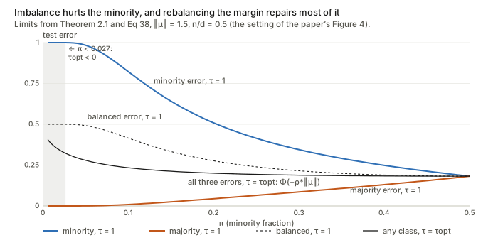
Proposition D.7 then shows the common error \Phi(-\rho^*\lVert\mu\rVert) falls in \pi, \lVert\mu\rVert and \delta. The proof reduces to monotonicity of \rho^* (Lemma G.2), itself read off Eq 76a with Lemmas G.6 and G.7 (both about ratios of g_1,g_2, shown by Mills-ratio calculus).
Theorem 3.2: the high-imbalance regime
Let \pi\asymp d^{-a}, \lVert\mu\rVert^2\asymp d^b and n\asymp d^{c+1}, so the minority sample is n_+\asymp d^{1+c-a} (it must grow, so a-c<1). Take \tau=d^r. The paper’s proof (App H, about 15 pages) rests on one idea, and the idea is simple.
The margin is at most half the distance between the two training class means (Lemma H.1). A minimum is at most an average, so at \tau=1 \kappa\le\tfrac12\big(\text{mean minority margin}+\text{mean majority margin}\big)=\tfrac12\langle\bar x_+-\bar x_-,\beta\rangle\le\tfrac12\lVert\bar x_+-\bar x_-\rVert. Now \bar x_+-\bar x_-=2\mu+\bar z_+-\bar z_-, and \lVert\bar z_+\rVert^2\approx d/n_+. So
\kappa\ \lesssim\ \sqrt{\lVert\mu\rVert^2+\tfrac{d}{4n_+}}\ \asymp\ \sqrt{d^{\,b}+\tfrac14 d^{\,a-c}},
and a constructed classifier along \bar
x_+-\bar x_- nearly attains it. asymptotics.py §8
checks the half-distance: 2.87 against 2.82 at d=500, and 3.64 against 3.56 at d=2000. Two lengths compete: the signal d^{b/2} and the minority’s
memorisable noise \sqrt{d/n_+}=d^{(a-c)/2}. The learned
direction has cosine \rho\approx
d^{b/2}/\sqrt{d^b+d^{a-c}/4} with \mu. Every minority training point
gets an extra logit of about d^{(a-c)/2} from the \bar z_+ component, and a test point gets
none. The intercept balances training margins, so it absorbs that
memorised boost (Lemma H.5):
\hat\beta_0\approx\Big(1-\frac{2}{\tau+1}\Big)\hat\rho\lVert\mu\rVert-\frac{1}{\tau+1}\sqrt{d/n_+}.
The minority’s test centre \hat\rho\lVert\mu\rVert+\hat\beta_0 must go to +\infty, and so must the majority’s \hat\rho\lVert\mu\rVert-\hat\beta_0. Comparing exponents gives the three phases:
| phase | condition | \hat\rho\lVert\mu\rVert | what works |
|---|---|---|---|
| high signal | a-c<b | \approx d^{b/2}, signal dominates | any 1\le\tau\ll d^{b/2} |
| moderate | b<a-c<2b | \approx2d^{\,b-(a-c)/2}\to\infty | only d^{\,a-b-c}\ll\tau\ll d^{(a-c)/2}; at \tau\asymp1, \mathrm{Err}_+\to1 |
| low signal | a-c>2b | \to0 | nothing: \mathrm{Err}_b\ge\tfrac12-o(1) |
In the moderate phase with \tau=1 the minority centre is roughly 2d^{\,b-(a-c)/2}-\tfrac12d^{(a-c)/2}, which goes to -\infty because b<a-c. Rebalancing divides the memorisation penalty by \tau+1. That fixes the minority once \tau\gg d^{\,a-c-b}, and it keeps the majority safe while \tau\ll d^{(a-c)/2}. Widget 4 of the interactive page draws the phase plane and the \tau window. The theorem extends to sub-Gaussian noise (Theorem D.8), since only norms and inner products of noise vectors enter.
Section 4: confidence and calibration
The confidence of the unit-norm SVM is \hat p(x)=\sigma(f(x)). Lemma I.1 gives the three probabilities in the limit. Only one derivation is needed, Bayes’ rule on the test logit. Given y, the logit f=\langle x,\hat\beta\rangle+\hat\beta_0 is \mathcal N(y\hat\rho m+\hat\beta_0,1). So
\log\frac{\mathbb P(y=+1\mid f)}{\mathbb P(y=-1\mid f)}=\log\frac{\pi}{1-\pi}+\frac{(f-\hat\beta_0+\hat\rho m)^2-(f-\hat\beta_0-\hat\rho m)^2}{2} =\log\frac{\pi}{1-\pi}+2\hat\rho m\,(f-\hat\beta_0),
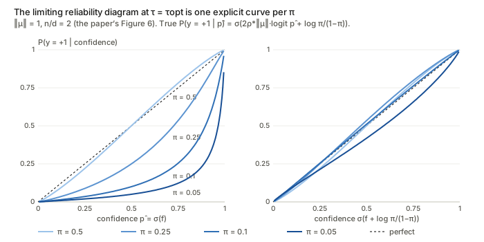
\hat p_0(x)=\mathbb P(y=1\mid\hat p(x))=\sigma\Big(2\rho^*\lVert\mu\rVert\,(f-\beta_0^*)+\log\tfrac{\pi}{1-\pi}\Big). \qquad\text{(Eq 173)}
The Bayes posterior is the same formula with the true direction: p^*(x)=\sigma(2\langle x,\mu\rangle+\log\frac{\pi}{1-\pi}). Proposition D.9 then writes \mathrm{CalErr}^*, \mathrm{MSE}^* and \mathrm{ConfErr}^* as one-dimensional Gaussian integrals. It proves that at \tau=\tau^{\rm opt}>0 the MSE (Brier score) \mathbb E[(1+e^{\rho^*m+G})^{-2}] falls in \pi, \lVert\mu\rVert and \delta, because it depends on them only through \rho^*\lVert\mu\rVert. The monotonicity of CalErr and ConfErr (Claim D.10) is checked numerically, not proved.
So the limiting reliability diagram is a closed-form curve: plot \hat p_0 against \hat p=\sigma(f). My numbers reproduce the CalErr values printed in the paper’s figures: Figure 6’s 0.001, 0.04, 0.12, 0.18 against my 0.0006, 0.041, 0.117, 0.163, and Figures 10 and 11 likewise (§7). So the figures are these curves plus binning noise.
Section 5: extensions, in brief
- Heterogeneous covariances \mathcal N(\pm\mu,\Sigma_\pm) with commuting \Sigma_\pm (Conjecture D.12): the ELD would be \max\{\kappa^*,\rho^*\lVert\mu\rVert+\sigma^*(Y)G+Y\beta_0^*\}. Each class keeps its own spread, and the truncation stays. For \Sigma_\pm=\sigma_\pm^2I, \sigma^*(Y)=\sigma_Y.
- Spiked covariances and K classes: Conjectures D.13 and D.11. The K-class one, derived with the non-rigorous replica method, predicts a Gaussian in \mathbb R^K projected onto a convex polytope. Figure 7 shows the two-hyperplane truncation for three classes on synthetic data and on CIFAR-10.
- Real data (Figures 2, 3): linear probes on RNA-seq, CIFAR-10/ResNet-18, IMDb/BERT and Llama-3-8B heads on TruthfulQA all show a truncated training histogram against a Gaussian-looking test histogram.
Questions and doubts
1. \tau^{\rm opt} is negative in several of the paper’s own experimental settings
Propositions D.7 and D.9(b), and Claim D.10, assume \tau=\tau^{\rm opt}>0. From Eq 38, \tau^{\rm opt}>0 iff \beta_0^*(1)+\kappa^*(1)>0. Otherwise the
balanced-error boundary lies beyond the majority’s support vectors, and
some majority training points are misclassified.
asymptotics.py §7 finds:
- Figure 6 (\lVert\mu\rVert=1, n/d=2): \tau^{\rm
opt}>0 only for \pi>0.227.
The panels at \pi=0.1 and 0.05 have \tau^{\rm
opt}=-8.8 and -7.1.
svm_simulation.py§4 confirms it at finite n: two draws give \hat\beta_0+\hat\kappa=-0.15 and -0.21 (the limit is -0.197). So no \tau>0 puts the boundary at \beta_0=0. - Figure 11 (\lVert\mu\rVert=0.5, n/d=2): negative at \pi=0.25, 0.1 and 0.05.
- Figures 4 and 9 (n/d=0.5): negative for \pi below 0.036, 0.027 and 0.020 at \lVert\mu\rVert=1.25,1.5,1.75. These figures plot \pi down to near 0.
The printed CalErr values match the \beta_0^*=0 formula, so the experiments presumably set \beta_0=0 directly, which is legitimate. Remark G.1 says the theory extends to \tau<-1 if the SVM is redefined, and Remark D.3 calls these cases “near-degenerate”. But half the reliability panels are in that regime, and the statements proved in Section D.3 do not cover them. The main text does not mention this.
2. The π-trend in calibration is mostly the discarded prior, not overfitting
Section 4 says parameter changes that raise test error “simultaneously worsen model calibration, revealing an adverse effect of overfitting”. Look at Eq 173 at \beta_0^*=0. The classifier’s confidence is \sigma(f), and the truth is \sigma(2\rho^*\lVert\mu\rVert f+\log\frac{\pi}{1-\pi}). There are two mismatches. One is the slope 2\rho^*\lVert\mu\rVert against 1. That is a question of scale, and it depends on the arbitrary normalisation \lVert\beta\rVert=1. The other is the prior log-odds, which rebalancing throws away on purpose to equalise the errors. Adding \log\frac{\pi}{1-\pi} back:
| setting | \pi | slope 2\rho^*\lVert\mu\rVert | \mathrm{CalErr}^* | after adding the prior |
|---|---|---|---|---|
| Fig 6, \lVert\mu\rVert=1 | 0.50 / 0.25 / 0.10 / 0.05 | 1.16 / 1.12 / 1.02 / 0.89 | 0.0006 / 0.041 / 0.117 / 0.163 | 0.0006 / 0.0003 / 0.0000 / 0.0001 |
| Fig 11, \lVert\mu\rVert=0.5 | same | 0.36 / 0.34 / 0.30 / 0.25 | 0.015 / 0.075 / 0.174 / 0.221 | 0.015 / 0.013 / 0.007 / 0.003 |
| Fig 10, \lVert\mu\rVert=2 | same | 3.27 / 3.25 / 3.19 / 3.13 | 0.025 / 0.031 / 0.044 / 0.053 | 0.025 / 0.027 / 0.024 / 0.016 |
In Figures 6 and 11 the prior accounts for 83–100% of the miscalibration at \pi\le0.25. With the prior restored, calibration actually improves as \pi falls. What remains is the slope, and it is unrelated to \pi. Separately, a logistic probe trained to convergence has \lVert\hat\beta\rVert\to\infty and confidences near 0 or 1, so the unit-norm SVM’s calibration is not that of the models the paper motivates with. The MSE result (Proposition D.9(b)) is fine, but it does not isolate overfitting either: it is a function of \rho^*\lVert\mu\rVert, i.e. of the test error.
3. “Truncation solely explains overfitting” on real data is shown, not tested
Figures 2 and 3 overlay histograms by eye. The features are not isotropic Gaussians, the classes need not have equal spread, and the logistic probes are fitted with L-BFGS, with a small ridge (C=10^6–10^8) added when they do not converge, so they are only approximately at the max-margin limit. A quantitative check would be to fit (\rho,\beta_0,\kappa) from the test logits, predict the training histogram (for example its support-vector fraction), and report W_2 or a KS distance. The theory makes a very specific prediction, a point mass at \kappa plus an untouched Gaussian tail, and it could have been tested as sharply as it is stated.
4. The extensions in Section 5 are conjectures
The main text says “our theory and proof strategies can also extend to non-isotropic settings … full theoretical statements are deferred to Appendix D.4”. But D.4 contains Conjectures D.11–D.13, not theorems; the multiclass one comes from the non-rigorous replica method. Even the heterogeneous case \Sigma_\pm=\sigma_\pm^2I quoted in the main text is a special case of Conjecture D.12. Only the sub-Gaussian extension of the high-imbalance theorem (D.8) is proved.
5. Smaller points
- Eq 28 prints +G inside (s(Y)\kappa-\rho\lVert\mu\rVert+G-Y\beta_0)_+. Everywhere else it is -G. Since G is symmetric this is harmless.
- Appendix A says “\phi and \Phi denote the CDF and PDF” (reversed). In Lemma E.1, Z_- is defined with rows where y_j=+1 (should be -1). In the proof of Lemma C.3, \langle x_{sv+}-x_{sv+},\beta\rangle should be \langle x_{sv+}-x_{sv-},\beta\rangle.
- Proposition D.2 (optimal transport) is true of any monotone map between 1-D laws, as noted above. “Optimal transport perspective” suggests more than it delivers.
- Theorem 3.2’s statements are rates with unspecified constants. At the d=2000 of Figure 5 the phase boundaries are necessarily blurred, and the figure reads more crisply than a finite-d experiment can.
What would settle it
For point 1, the paper would need to report the \tau actually used in Figures 4, 6, 9 and 11, and either restrict \pi to the \tau^{\rm opt}>0 range or state the extension to \tau<-1 as a theorem. For point 2, compare the calibration of \sigma(f+\log\frac{\pi}{1-\pi}) with that of \sigma(f), and separate the “scale” part from the “prior” part. For point 3, fit the three parameters on held-out logits and test the predicted training histogram.
Takeaways
- Overfitting in a linear probe has a shape. Training logits are test logits with the part below the margin moved onto the margin. The support vectors are that atom, and their fraction per class is \Phi(\kappa^*-\text{class centre}).
- The mechanism is a budget. The d free directions can lift n training logits by a mean square of (1-\rho^2)/\delta. The cheapest way to spend it is truncation. Gordon’s theorem turns this heuristic into an exact statement: separability at margin \kappa iff \delta\,\mathbb E(s\kappa-X)_+^2\le1-\rho^2.
- The minority suffers because both classes get the same total push. So each minority point gets (1-\pi)/\pi times more, the intercept shifts towards the minority, and the minority’s test Gaussian ends up nearer the boundary.
- Rebalancing moves only the intercept, exactly and in finite samples. \tau^{\rm opt} has a closed form, but it can be negative. That happens whenever the balanced boundary would have to cross the majority’s margin, which occurs in several of the paper’s own settings.
- Calibration claims depend on the prior and the scale. The limiting reliability diagram is the explicit curve \sigma(2\rho^*\lVert\mu\rVert f+\log\frac{\pi}{1-\pi}) against \sigma(f). Most of its dependence on \pi disappears once the prior log-odds are added back.