Dynamics and Reachability of Learning Tasks
Links
- arXiv:1810.02440:
the preprint;
pdf_urlpoints here. The version annotated is v2 (29 May 2019, 9 pages, marked “under review”). There is no appendix: every derivation is in the main text. - Interactive companion: particles escaping over a barrier while you move the end point; particles in a valley with a sharp and a flat minimum, against three effective potentials; Figure 2’s two matrices as a clickable scatter; the batch-size curve of a noise floor; and the structure function with a slider for \beta (eqs. 2–3).
- Questions from a first reading, the first section after the spine: what the transition probability, the information-theoretic distance and reachability are; eqs. (2), (3), (5) and (9) and the SDE line by line; the Fisher in place of the Hessian; and two comments, on feature-only transferability scores and on dataset against architecture.
- Runnable
code: every number on this page, and the six figures
(
python3 reachability.py --figures).make verifyruns it, in about four seconds. - Background: Langevin dynamics, for the Gibbs law, Fokker–Planck, Kramers’ law, detailed balance and the path weight used throughout, built up from scratch with simulations; and Inequalities and concentration, for the KL divergence and the Donsker–Varadhan formula, which is the identity that makes Section 6 work.
- Fisher information: background for the Fisher matrix used in eq. (4) in place of the Hessian: the score, Cramér–Rao, the local KL expansion, Hessian against Fisher against empirical Fisher, and natural gradient.
- Transferability: the site’s section on estimating how well fine-tuning from a source will work without running it (LEEP, NCE, LogME, H-score, SFDA, PAS, and two evaluations on medical targets). Those scores and this paper ask the same question from opposite ends: they score frozen features, and this paper models the fine-tuning dynamics. The question on feature-only scores below places each of them against the paper’s two factors.
- The static distance of Section 4 comes from a companion paper, Achille, Paolini, Mbeng & Soatto, The Information Complexity of Learning Tasks, their Structure and their Distance (arXiv:1904.03292).
In one paragraph
The paper asks how hard it is to fine-tune: starting from weights that solve task A, how likely is SGD to reach weights that solve task B, and how long does it take? It models SGD as a particle rolling downhill on the loss while being kicked by noise (a Langevin equation), writes the probability of every possible training trajectory as a path integral, and splits the probability of getting from w_0 to w_f into two factors. The static factor e^{-\Delta U/2D} depends only on the loss at the two end points. The reachability factor measures whether likely paths connect them. Integrating out the directions across a valley adds a curvature term to the loss, U_{\text{eff}}=U+D\log\lvert H\rvert, which with weight decay and a Gaussian prior the paper identifies with the task’s information complexity C_\beta from a companion paper. The conclusion is a Kramers-type law, waiting time \propto e^{\Delta C_\beta/D}, tested on random labels, batch sizes and an 8\times8 matrix of fine-tuning times. The machinery is right in outline, and one part of it checks out better than the paper shows. The static/reachability split is exactly detailed balance: the reachability factor is symmetric in the two end points, so for a fixed loss all the asymmetry of a transition lives in the static factor. Several constants are off: the curvature term is (D/2)\log\lvert H\rvert, and the identification with C_\beta holds exactly, for every posterior and not just Gaussians, when \beta=D and \lambda^2=D/\gamma, not \beta=2\lambda^2\gamma. The central law, eq. (16), is not Kramers’ law: escape times follow the height of the barrier to the saddle, not the difference between the two end points (checked below: moving that difference over a range of 1.9 at a fixed barrier leaves the escape time essentially unchanged). On the most likely downhill path the static factor is cancelled exactly by the dynamic one, so “upper-bounded by the static part” says nothing in the fine-tuning direction. Re-reading Figure 2 from its printed numbers, the static distance does rank sources for a fixed target (within-target r=0.58), which is better support than the paper’s pooled scatter gives.
The spine of the argument
- SGD is a noisy gradient flow (§2). In the small-step limit, \dot w=-\nabla U(w)+\sqrt{2D}\,n(t), with white noise n and a temperature D\propto\eta/B.
- A task’s complexity (§3–4). The structure function trades off training loss against the information stored in the weights. Its Lagrangian C_\beta=\mathbb E_Q[L]+\beta\,\mathrm{KL}(Q\Vert P), evaluated with Gaussians, becomes loss plus a log-determinant of the Hessian (eq. 4). The static distance d_\beta(\mathcal D_1\to\mathcal D_2) is how much C_\beta grows when \mathcal D_2 is added to \mathcal D_1.
- Path integral (§5). Each trajectory w(t) gets a weight e^{-S[w]} (Onsager–Machlup). A Stratonovich chain rule pulls \Delta U out of the action, giving static \times reachability (eq. 10).
- Most likely paths and the valley (§5.2). The saddle-point approximation keeps only critical paths. Integrating out the transverse directions of a valley corrects U by a curvature term (eqs. 11–14).
- Curvature is complexity (§6). With weight decay \gamma the corrected potential looks like C_\beta of eq. (4), so the static factor becomes e^{-\Delta C_\beta/2D} (eq. 15) and the convergence rate e^{-\Delta C_\beta/D} (eq. 16).
- Experiments (§7). Convergence time grows with the number of random labels and with the estimated complexity, falls with batch size, and fine-tuning time grows with the static distance.
Questions from a first reading
Twelve questions and comments from a first pass through the paper, answered in the order they were asked. Each answer starts with the idea in plain words, then gives the formula, then a number from the code where one helps. The sections after this one go through the same material in the paper’s order. The Langevin dynamics foundations page builds the physics (noise, the Gibbs law, Kramers’ law, path weights) from scratch.
What is the transition probability?
Start SGD many times from the same weights w_0, for example the solution of a pre-training task. The runs see different mini-batches, so they follow different paths and, after a training time t, end up at different weights. The transition probability p(w_f,t\mid w_0) is the density of where they end up: how likely it is, per unit volume of weight space, that SGD started at w_0 is at w_f after time t. It is a conditional density in w_f, so it integrates to 1 over w_f. For fine-tuning, w_0 is the source solution and the question “does fine-tuning reach a good target solution within the budget?” is the integral of p(w_f,t\mid w_0) over the region of good target solutions.
Two limits make it concrete. At t\to0 it is a spike at w_0: nothing has moved. As t\to\infty it forgets w_0 and becomes the stationary (Gibbs) law \propto e^{-U/D}. Everything interesting is in between. In the code’s tilted double well (§5 below), the probability of being within 0.1 of the lower well, starting in the upper one, is 9\times10^{-5} at t=0.5, 0.052 at t=5, 0.29 at t=50 and 0.33 at t=500. Eq. (7) computes it as the total weight of all paths from w_0 to w_f (answer to eq. 5 below).
What is the information-theoretic distance?
It is the extra cost of explaining a second dataset once you can explain the first:
d_\beta(\mathcal D_1\to\mathcal D_2)=C_\beta(\mathcal D_1\cup\mathcal D_2)-C_\beta(\mathcal D_1),
where C_\beta(\mathcal D) is the smallest value of “training loss +\;\beta\times nats stored in the weights” over all ways of fitting \mathcal D (eq. 3, below). It is information-theoretic because the nats are a description length: \mathrm{KL}(Q\Vert P), the number of nats needed to write down the trained weights (as a cloud Q) given the prior P. If \mathcal D_2 adds little that the model for \mathcal D_1 does not already encode, the distance is small. It is asymmetric by design: CIFAR-100 \to CIFAR-10 is 0.01 in Figure 2 and CIFAR-10 \to CIFAR-100 is 0.52, because knowing 100 classes already covers 10, not the other way round. It is not a distance in the metric sense (it can be negative with the paper’s averaged loss, §4). It comes from the companion paper; the task-complexity notes go through its definition, Lemma 4.2 and the identity that makes its asymmetry a difference of complexities. In practice the paper evaluates it with eq. (4): loss, weight norm and the log-determinant of the Fisher, at trained weights. It is called static because it says nothing about how SGD gets from one solution to the other.
“The takeaway: landscape geometry, and the ease of traversing the path”
Yes, that is the paper’s own two-factor message (eq. 10), and it holds up, with one refinement about how the work divides between the factors.
- The static factor depends only on the heights of the start and end points: the loss, corrected for curvature. It turns out to be exactly half the equilibrium log-odds between them, which is detailed balance (§5). So it decides which direction is favoured, not how fast anything happens.
- The ease of traversal, the reachability factor, carries all the time dependence: barriers, narrow passes, and whether a likely path exists within the training budget. The escape time follows the barrier exponentially (§6: d\ln\tau/d(1/D) equals the barrier height, 0.998 against 1, whatever the end points), and on the most likely downhill path the static factor is cancelled exactly (§5).
A sharper takeaway: fine-tuning is easy when the target’s loss has a low-barrier path from the source solution into a good target basin, and the information-theoretic distance is a proxy for that. The proxy works better than one might expect: within a fixed target, it ranks sources with r=0.58 (§7).
What does reachability mean?
A target solution is reachable from w_0 in time t if some likely SGD paths of that duration connect them. Formally it is the second factor of eq. (10), the path integral
K_t(w_0\to w_f)=\int e^{-\frac1{2D}\int_0^t\left[\frac12\lVert\dot w\rVert^2+V(w)\right]ds}\,\mathcal Dw ,
the total weight of all paths from w_0 to w_f after the end-point factor is taken out. It is large when there are many short, low paths, and tiny when every path must climb a barrier or squeeze through a narrow pass. It depends on the time budget: at short times only nearby points are reachable, and given long enough everything is. It is also symmetric, K_t(a\to b)=K_t(b\to a) (§5).
“Unreachable” in practice means that the expected time to get there, which grows like e^{\text{barrier}/D}, is far longer than the training run. The paper’s motivating example is its reference [3], critical learning periods: a network first trained on blurred images never recovers full performance, although the good solution exists. In Figure 2 the one visible case is MNIST \to Letters, which never converged although its static distance (0.68) is smaller than that of Fashion \to Letters (0.72, converged in 79.7 epochs).
“Transferability scores use only features; open-weight models come without data”
Both halves are right, and the second is worth separating by which quantity needs which data.
- What the usual scores do. LEEP, NCE, LogME, H-score, SFDA and PAS pass the target data through the frozen pre-trained model once and score how well its features (or its source-label predictions) fit the target labels. They need only the weights and the target data, and they implicitly model a linear probe: the features do not move. Fine-tuning is exactly the part where they move.
- What this paper needs. The static distance needs the source dataset: C_\beta(\mathcal D_1\cup\mathcal D_2)-C_\beta(\mathcal D_1) trains on \mathcal D_1 and on the union. For an open-weight model released without its data that is not computable.
- The dynamic side does not need the source data. Fine-tuning runs SGD on the target loss, starting from the released weights w_0. Everything in the reachability factor is a property of the target loss around w_0: its value and gradient there, its curvature (the target Fisher at w_0, which is what the paper’s reference [1], Task2Vec, computes with a probe network), the barriers between w_0 and target basins, and the neural tangent kernel of w_0 on target data (the NTK-selector and Fort et al. notes). A dynamics-aware score from weights plus target data alone is therefore possible in principle. What is lost without the source data is the static term, which by the detailed-balance argument is the factor that says least about speed anyway.
That is a suggestion, not a result of the paper; it has not been tested here.
Where each score in the Transferability section sits against the two factors. All of them are static in the paper’s sense: none models a path.
| Score | What it measures | What it needs | Relation to this paper |
|---|---|---|---|
| NCE | conditional entropy of the target labels given the source model’s predicted labels | source-model predictions and target labels | a data-level distance between label sets, with no training |
| LEEP | likelihood of the target labels under a classifier built from the source model’s soft predictions | the same | static, one hand-built classifier instead of the best one |
| LogME | evidence of the target labels for a Bayesian linear head on frozen features | features and target labels | exactly the paper’s complexity \min_QC_\beta of the target task, restricted to the last layer (at \beta=1 with a summed loss, \beta=1/N with the paper’s average; see the task-complexity notes) |
| H-score | how much of the feature covariance the target class means explain | features and target labels | static |
| SFDA | class separability in a Fisher-discriminant projection, after deliberately making the target task harder | features and target labels | static, with a heuristic meant to imitate fine-tuning: the closest any of them comes to the dynamic factor |
| PAS | a nearest-centroid margin of the target features | features and target inputs, no target labels | static |
| Chaves et al., Claßen et al. | evaluations of these scores on medical targets | — | the rankings do not carry over to medical tasks and are not stable across random seeds: evidence that frozen-feature scores miss part of what decides fine-tuning |
Two differences from the paper’s static distance stand out. The scores need only the target data, while d_\beta(\mathcal D_1\to\mathcal D_2) also needs the source data. And LogME, the one that coincides with the paper’s complexity, scores the target alone, C_\beta(\mathcal D_2), not the extra complexity C_\beta(\mathcal D_1\cup\mathcal D_2)-C_\beta(\mathcal D_1) on top of the source.
The structure of a task, nuisance against task-relevant information, and eq. (2)
The idea. A dataset contains two kinds of information. Structure is what many samples share: that cats have pointed ears, that digits are strokes. One nat of it lowers the loss on many samples at once. Nuisance is what is particular to individual samples: the exact background of image 4 017, a mislabelled example. One nat of it lowers the loss on one sample. A model trained long enough stores both, and only the first generalises.
Eq. (2) measures this with a budget:
S_{\mathcal D}(t)=\min_{Q:\ \mathrm{KL}(Q\Vert P)<t}\ \mathbb E_{w\sim Q}\big[L_{\mathcal D}(w)\big].
Piece by piece:
| Piece | Meaning |
|---|---|
| P(w) | the prior: what the weights look like before any data, e.g. \mathcal N(0,\lambda^2I) |
| Q(w) | a “posterior”: a cloud of weights around the trained solution, not a single point, because exact real numbers take infinitely many bits |
| \mathrm{KL}(Q\Vert P) | the number of nats needed to describe the cloud Q to someone who knows P: the information stored in the weights |
| \mathbb E_{w\sim Q}[L_{\mathcal D}(w)] | the average training loss of weights drawn from the cloud |
| S_{\mathcal D}(t) | the best training loss achievable with at most t nats: the structure function |
S_{\mathcal D} falls as t grows. It falls fast while the nats buy structure, then slowly once the only thing left to buy is nuisance, one sample at a time. The knee between the two regimes is the point to stop.
On a model that can be solved exactly. The code builds linear regression with N=100 samples and 50 weight directions: 5 strong input directions carry the true weights, 45 weak ones carry only label noise. For a quadratic loss the best Q at every budget is Gaussian and known in closed form, so the whole curve is exact.
- Storing everything (memorising): 570.7 nats, training loss 0.250, test loss 0.745.
- The best test loss, 0.588, needs only 24.7 nats. 16.2 of them go to the 5 signal directions and 8.5 to the other 45.
- Memorising spends 539.1 of its 570.7 nats on the 45 noise directions: that is the nuisance.
- With random labels there is no structure to find. The test loss is lowest at 18 nats (12.02), the cost of learning that the weights should be near zero. Memorising takes 9 954 nats and raises the test loss to 16.71.
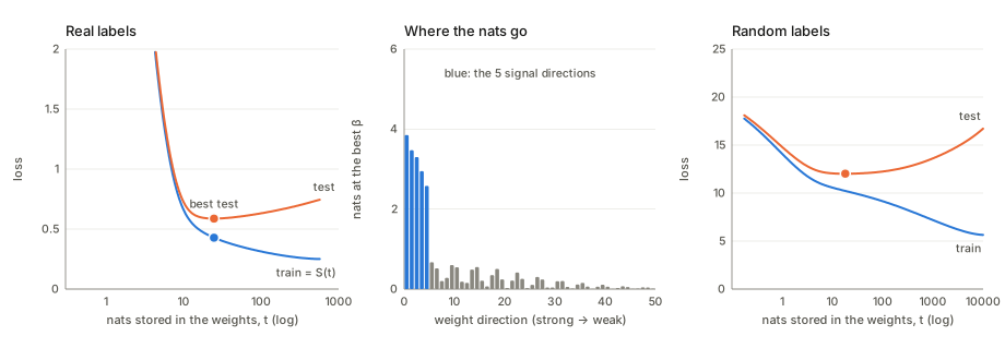
The paper’s eq. (2) is a continuous version of Kolmogorov’s structure function from algorithmic information theory; the task-complexity notes cover Kolmogorov’s discrete version, random labels (every nat is nuisance) and why only the convex hull of S matters.
“The dataset, not the architecture, dictates transferability”
That is plausible for a fixed, reasonably good architecture, but this paper cannot decide it, and some evidence points the other way.
- For the dataset. Re-read from Figure 2’s printed matrices (§7), the identity of the target explains a lot: row means of the distance and of log-epochs correlate at 0.75, since Letters takes 53–80 epochs from any source and MNIST under 1. Within a target, the source dataset still matters (r=0.58).
- But Figure 2 uses one architecture (ResNet-18) throughout, so it holds the architecture fixed and cannot measure its effect.
- For the architecture. Figure 1 (right) shows convergence time against complexity for three architectures, and the slopes differ several-fold. The paper itself says the dynamic factor “depends on the architecture of the network”. Even the static distance is computed through a ResNet-18’s Fisher, so in practice it depends on the probe network. Outside this paper, Kornblith, Shlens & Le (Do Better ImageNet Models Transfer Better?, CVPR 2019) find that transfer tracks ImageNet accuracy across architectures, and that some training choices that raise ImageNet accuracy (label smoothing, dropout, auxiliary heads) make the frozen features transfer worse. The Chaves et al. and Claßen et al. notes show that which pre-trained model looks best changes with the target dataset: the two interact.
- In the paper’s own formalism the loss U(w) depends on the data through L_{\mathcal D} but on the architecture through the parameterisation. The same set of functions, parameterised differently, has different curvatures, barriers and gradient noise, so a different \log\lvert H\rvert and a different temperature D. Information stored in weights is not invariant to reparameterisation. The claim of §5.2 that reachability “to first approximation depends only on information-theoretic quantities” of the data is the step that removes the architecture, and it is the step this reading disputes.
A fair summary: the dataset pair probably sets most of the variation in which transfers are easy; the architecture sets the time scale and some of the ranking.
The Lagrangian, eq. (3)
Eq. (2) is a problem with a budget: “best loss using at most t nats”. Budgets are awkward to optimise. Eq. (3) replaces the budget by a price:
C_\beta(\mathcal D;P,Q)=\underbrace{\mathbb E_{w\sim Q}\big[L_{\mathcal D}(w)\big]}_{\text{error}}+\beta\,\underbrace{\mathrm{KL}(Q\Vert P)}_{\text{nats stored}} .
Each nat costs \beta units of loss, and the optimiser buys nats only while one more nat lowers the loss by more than \beta. It is the same choice as a phone plan with a data cap against one that charges per gigabyte. The multiplier \beta is the Lagrange multiplier of the budget constraint, and its meaning is exactly the exchange rate: at the optimum, one more nat of budget lowers the best loss by \beta, \beta=-dS_{\mathcal D}/dt.
Geometrically, minimising C_\beta slides a straight line of slope -\beta up from below until it touches the curve S_{\mathcal D}(t); the touching point is the solution. A small \beta (cheap nats) gives a flat line that touches far to the right: memorise. A large \beta gives a steep line that touches near t=0: store almost nothing. In the solvable model the code checks that the slope of S at each \beta-optimum is -\beta, to a relative error of 1.6\times10^{-4}, and the best test loss sits at \beta=4.8\times10^{-3}. The interactive page has a slider for it.
Three connections the paper mentions, in plain terms:
- the Q that minimises C_\beta over all distributions is the Gibbs posterior Q^*\propto P(w)\,e^{-L_{\mathcal D}(w)/\beta} (§6), and \min_QC_\beta=-\beta\log\int P\,e^{-L_{\mathcal D}/\beta};
- it is the PAC-Bayes objective, whose value bounds the test error;
- at \beta=1/N (not \beta=1, since L_{\mathcal D} is an average) it is minus the ELBO of variational inference, divided by N.
The “critical \beta” of the companion paper is where the touching point jumps from the structure part of S to the nuisance part.
The Fisher as a robust positive semi-definite approximation of H
Why an approximation is needed at all. Eq. (4) contains \log\big\lvert\frac{\lambda^2}\beta H+I\big\rvert and the posterior covariance \Sigma^*=\beta(H+\frac\beta{\lambda^2}I)^{-1}. Both make sense only if every eigenvalue of the Hessian H is above -\beta/\lambda^2. Away from a clean minimum, at a saddle or wherever the loss curves downward in some direction, H has negative eigenvalues, the matrix inside the log can have a negative determinant, and “the variance of the posterior” would be negative.
Why the Fisher is always safe. The Fisher information is an average of outer products,
F=\mathbb E_{x}\,\mathbb E_{y\sim p_w(y\mid x)}\big[\nabla_w\log p_w(y\mid x)\,\nabla_w\log p_w(y\mid x)^\top\big],
and for any direction v, v^\top Fv=\mathbb E[(v^\top\nabla\log p)^2]\ge0. So F is positive semi-definite at every w, whatever the network.
Why it is close to the Hessian. For cross-entropy with logits z_w(x), differentiating twice gives
H=\underbrace{\mathbb E_x\big[J^\top(\operatorname{diag}p-pp^\top)J\big]}_{=F\ \text{(Gauss–Newton)}} +\underbrace{\mathbb E_{x,y}\Big[\textstyle\sum_c(p_c-\mathbb 1[y=c])\,\nabla_w^2z_c\Big]}_{\text{residual}}, \qquad J=\partial z/\partial w .
The first term is the Fisher exactly, because the curvature of softmax cross-entropy in logit space, \operatorname{diag}p-pp^\top, does not depend on the label. The residual is weighted by the prediction errors p-e_y and by how curved the logits are in the weights. It vanishes for a model linear in its weights, and it is small near a good fit.
The code checks each claim on one-input logistic models with 400 points:
- logistic regression z=a+bx: \max\lvert H-F\rvert=0 over 200 random weight settings, since the logit is linear in the weights;
- the nonlinear model z=a\tanh(cx): over a grid of 961 weight settings in [-3,3]^2, the Hessian has a negative eigenvalue at 643 of them (as low as -1.211); the Fisher at none;
- at the fitted minimum the two nearly agree: eigenvalues 0.0092,0.0858 for H against 0.0083,0.0852 for F;
- at the worst grid point, with \beta=0.05, the matrix inside eq. (4)’s log has an eigenvalue of -23.2 with the Hessian and 1.035 with the Fisher.
Two cautions. The “empirical Fisher”, with the true labels in place of y\sim p_w, is a different matrix and not guaranteed to be close to H (the Fisher information page, §8, measures how far it strays). And on a trained network the relative gap between H and F stops shrinking at a few percent; the information-in-the-weights notes measure it (about 4%) in their section on Lemma 2.4. A bonus of the Fisher: because y is drawn from the model, it depends on the data only through the inputs, which is why it can be computed on a target task without its labels.
The stochastic differential equation \dot w=f(w)+\sqrt{2D}\,n(t)
Read it as a statement about velocity: the weights move with a deterministic push f(w) plus a random push.
| Piece | Meaning |
|---|---|
| f(w) | the drift, -\nabla U(w): downhill on the regularised loss (the paper writes +\nabla U, a sign slip) |
| n(t) | white noise: at every instant an independent standard Gaussian kick; formally the derivative of Brownian motion |
| D | the temperature: how strong the kicks are. For SGD, D=\eta\sigma^2/(2B) (learning rate \eta, gradient-noise variance \sigma^2, batch size B) |
| \sqrt{2D} | the factor that makes pure noise spread with variance 2Dt and the equilibrium come out as e^{-U/D} |
To simulate it, take small steps \eta: w\leftarrow w-\eta\nabla U(w)+\sqrt{2D\eta}\,\xi with \xi\sim\mathcal N(0,I). That is gradient descent plus a Gaussian kick after every step. The kick scales with \sqrt\eta, not \eta, because independent kicks add in variance. With kicks proportional to \eta the noise would vanish in the limit; the foundations page shows this numerically.
Where it comes from (§2 below): an SGD step is a full-gradient step plus the mini-batch error, which has mean zero and variance \eta^2\sigma^2/B per step. Matching that to the SDE’s 2D\eta gives D=\eta\sigma^2/(2B). The code confirms it on a toy loss: stationary variance 0.0187, 0.00471, 0.00115 for B=4,16,64 against D=0.0181,0.00453,0.00113.
What it predicts: the Gibbs law e^{-U/D} at equilibrium, escape times e^{\text{barrier}/D}, and a preference for flat minima through \frac D2\log\lvert H\rvert (§5–6).
What it assumes: small steps, Gaussian noise, and noise that is the same in every direction and at every w. Real SGD noise is shaped roughly like the Hessian and changes with w, which changes the equilibrium (foundations page, §7 and §10).
Eq. (5), line by line
Eq. (5) gives a probability to an entire training trajectory:
p(w(\cdot)\mid w_0,t_0)=e^{-S[w]}=\exp\Big(-\int_{t_0}^{t_f}\mathcal L(w,\dot w)\,dt\Big), \qquad \mathcal L=\frac1{4D}\lVert\dot w-f(w)\rVert^2+\frac12\operatorname{div}f(w).
Where it comes from. Chop the trajectory into steps of length \Delta t: positions w_0,w_1,\dots,w_n. Each step of the SDE is w_{k+1}=w_k+f(w_k)\Delta t+\sqrt{2D\Delta t}\,\xi_k. So a given path requires the kicks \xi_k=(w_{k+1}-w_k-f(w_k)\Delta t)/\sqrt{2D\Delta t}, and the probability of those kicks is a product of Gaussian densities:
\prod_{k}\frac{1}{\sqrt{4\pi D\Delta t}}\exp\Big(-\frac{(w_{k+1}-w_k-f\,\Delta t)^2}{4D\,\Delta t}\Big) =\big(4\pi D\Delta t\big)^{-n/2}\exp\Big(-\frac1{4D}\sum_k\Big(\frac{w_{k+1}-w_k}{\Delta t}-f\Big)^2\Delta t\Big).
The sum in the exponent is a Riemann sum for \frac1{4D}\int(\dot w-f)^2dt. The code checks the identity on a random 20-step path: the product of the step densities is 1.7210\times10^{-2}, and so is e^{-\text{action}}(4\pi D\Delta t)^{-n/2}.
How to read it. Every path has a cost S. A path that moves exactly with the drift, \dot w=f(w), needs no kicks and costs nothing. Every deviation costs its square, divided by 4D: at low temperature deviations are expensive and the likely paths hug gradient descent; at high temperature the particle wanders. The prefactor (4\pi D\Delta t)^{-n/2} blows up as \Delta t\to0, which is why only ratios of path weights and integrals over paths are meaningful, never the weight of one path on its own.
The \frac12\operatorname{div}f term is a correction of order 1 (the main term is of order 1/D). It comes from evaluating f at the midpoint of each step instead of the start, which is the reading that lets the chain rule of eq. (9) work. With f=-\nabla U, \operatorname{div}f=-\nabla^2U: where the loss curves upward, the flow squeezes nearby paths together, and the term raises the weight of paths through such regions.
Eq. (7) adds up all paths. The probability of being at w_f at time t is the total weight of every path that ends there. On a grid that sum is just the short-time transition matrix multiplied by itself n times, one factor per step. For the Ornstein–Uhlenbeck process, where the exact answer is known, the code finds maximum errors of 0.129, 0.025 and 0.0025 (against a peak density of 0.607) with 2, 10 and 100 steps. The sum over paths converges to the exact transition probability as the steps shrink.
Eq. (9), line by line
Eq. (9) splits the path weight of eq. (5) into a part that depends only on the end points and a part that depends on the whole path:
p(w(\cdot)\mid w_0)=\underbrace{e^{-\frac{1}{2D}[U(w_f)-U(w_0)]}}_{\text{end points only}}\; \underbrace{\exp\Big(-\frac1{2D}\int\Big[\tfrac12\lVert\dot w\rVert^2+V(w)\Big]dt\Big)}_{\text{the whole path}}, \qquad V=\tfrac12\lVert\nabla U\rVert^2-D\,\nabla^2U .
The algebra, with f=-\nabla U:
- Expand the square: \frac1{4D}\lVert\dot w+\nabla U\rVert^2=\frac1{4D}\lVert\dot w\rVert^2+\frac1{2D}\nabla U\cdot\dot w+\frac1{4D}\lVert\nabla U\rVert^2.
- The middle term is a total derivative: \nabla U\cdot\dot w=\frac{d}{dt}U(w(t)) by the chain rule, so its integral is U(w_f)-U(w_0) whatever the path. That is the static factor.
- The divergence term \frac12\operatorname{div}f=-\frac12\nabla^2U joins the rest. Collecting everything that is left, \frac1{4D}\lVert\dot w\rVert^2+\frac1{4D}\lVert\nabla U\rVert^2-\frac12\nabla^2U=\frac1{2D}\big[\frac12\lVert\dot w\rVert^2+V\big].
What it means.
- The second factor does not change if the path is run backwards in time (\lVert\dot w\rVert^2 and V(w) do not care about direction). So all the difference between going a\to b and b\to a is in the first factor: p_t(b\mid a)/p_t(a\mid b)=e^{-[U(b)-U(a)]/D} at every t. That is detailed balance. The code measures the ratio at 7.403 at t=0.5, 5, 50 and 500, against e^{-\Delta U/D}=7.395 (the gap is the grid).
- V is an “effective potential” felt by paths: it is high where the loss is steep, so a path that lingers on a slope without moving with it is penalised, and it is lowered by curvature.
- The two factors are not independent. Along the most likely downhill path the first factor is e^{+\lvert\Delta U\rvert/2D} and the second is exactly e^{-\lvert\Delta U\rvert/2D}: the code finds -1.2616+1.2616=0 (§5). Going uphill they multiply to e^{-\Delta U/D}. So “energy gap times existence of paths” is a correct factorisation but not a separation of causes. The static factor tells you the odds of the two directions, and the path factor tells you how long you will wait.
Setup and notation
| Symbol | Meaning |
|---|---|
| \mathcal D=\{(x_i,y_i)\}_{i=1}^N | a training set; a task is a dataset plus a loss |
| p_w(y\mid x) | the network’s predicted label distribution with weights w\in\mathbb R^k |
| L_{\mathcal D}(w) | cross-entropy, averaged over the N samples (this matters twice below) |
| U(w)=L_{\mathcal D}(w)+\frac\gamma2\lVert w\rVert^2 | the loss with weight decay \gamma: the “potential” the particle rolls on |
| \eta, B | learning rate and batch size |
| D | the diffusion constant (temperature) of SGD, D=\eta\sigma^2/(2B) for gradient-noise variance \sigma^2 |
| n(t) | white noise: independent standard Gaussian kicks at every instant |
| P(w)=\mathcal N(0,\lambda^2 I) | the prior over weights |
| Q(w\mid\mathcal D)=\mathcal N(w_0,\Sigma) | a “posterior”: a cloud of weights around w_0 |
| C_\beta | \mathbb E_Q[L_{\mathcal D}]+\beta\,\mathrm{KL}(Q\Vert P), error plus \beta times information |
| H, F | Hessian of L_{\mathcal D}; Fisher information matrix |
| \lvert H\rvert, \lvert H\rvert_+ | determinant; product of the positive eigenvalues only |
| S[w], \mathcal L(w,\dot w) | the action of a path and its Lagrangian: the path’s weight is e^{-S} |
| V(w) | the “effective potential” of eq. (8), \frac12\lVert\nabla U\rVert^2-D\,\nabla^2U |
| \nabla^2U | the Laplacian, \operatorname{tr}H_U: total curvature |
| \tau, 1/\tau_K | mean time to reach the target; the Kramers rate |
§2 SGD as a noisy particle
From the update rule to a Langevin equation
A mini-batch gradient is the full gradient plus a zero-mean error, so an SGD step is a gradient-descent step plus a random kick:
w_{k+1}=w_k-\eta\nabla\hat L_{\xi_k}(w_k) =w_k-\eta\nabla L(w_k)-\underbrace{\eta\big(\nabla\hat L_{\xi_k}-\nabla L\big)}_{\text{mean }0,\ \text{covariance }\eta^2\Sigma/B}.
Read the step index as time, t=k\eta. Over one step of length \eta the drift is -\eta\nabla L and the kick has variance \eta^2\sigma^2/B per coordinate (for isotropic \Sigma=\sigma^2 I). A diffusion \dot w=-\nabla L+\sqrt{2D}\,n(t) has kick variance 2D\eta over the same time. Matching the two gives
D=\frac{\eta\,\sigma^2}{2B},
which is the paper’s D\propto\eta/B. The code checks it on SGD for the toy per-sample loss \frac12(w-z_i)^2 (Hessian 1, \sigma^2=2.90, \eta=0.05). The stationary variance of w should be D, and it is: 0.0187, 0.00471, 0.00115 against D=0.0181, 0.00453, 0.00113 for B=4, 16, 64. The 3% excess is the finite-step correction; the exact value for this linear recursion is \eta\sigma^2/(B(2-\eta)), and it matches to within Monte Carlo error.
Two things about how the paper writes it.
- Eq. (1) as printed is plain gradient descent. It reads w_{k+1}=w_k-\eta\nabla\hat L_{\xi_k}(w_k)+\sqrt\eta\,T_{\xi_k} with T=\sqrt\eta(\nabla\hat L_{\xi_k}-\nabla L). Substituting, the mini-batch gradient cancels and what remains is w_k-\eta\nabla L(w_k): the noise is added and then removed. The drift should be the full gradient, w_{k+1}=w_k-\eta\nabla L(w_k)-\sqrt\eta\,T_{\xi_k} (the code checks both to machine precision). A typo, but it is the equation the whole model rests on.
- “D=k/B with k a constant that depends on the architecture.” The constant is \eta\sigma^2/2. The gradient-noise variance \sigma^2 depends on the data, the loss and the current weights, and the noise is neither isotropic nor constant (the paper says so, then sets that aside).
The Fisher information
A small change \delta w of the weights changes the predicted label distributions by
\mathbb E_x\,\mathrm{KL}\big(p_w(y\mid x)\,\Vert\,p_{w+\delta w}(y\mid x)\big)=\tfrac12\,\delta w^\top F\,\delta w+o(\lVert\delta w\rVert^2),
with a factor \tfrac12 that the paper omits (it also calls the left side F, the same letter as the matrix). On a softmax regression the ratio of the two sides is 0.5027, 0.4996, 0.5000 for \lVert\delta w\rVert=10^{-1},10^{-2},10^{-3}. The paper’s other remark is correct and worth keeping: the Fisher uses labels drawn from the model, y\sim p_w(y\mid x), so it depends on the data only through the inputs x. That is why it can stand in for the Hessian later without seeing the labels.
§3 The structure function: error against bits
The structure function of a dataset asks: if you may store at most t nats of information in the weights, how low can the average training loss go?
S_{\mathcal D}(t)=\min_{\mathrm{KL}(Q\Vert P)<t}\ \mathbb E_{w\sim Q}\big[L_{\mathcal D}(w)\big].
Why a distribution Q over weights and not one weight vector: writing down a real-valued vector exactly takes infinitely many bits. A “noisy” weight, a cloud Q around w_0, can be described with finitely many bits relative to a prior P, and \mathrm{KL}(Q\Vert P) is that description length. Think of a rate–distortion curve. The first few nats buy large drops in loss (the task’s structure). Later nats buy less and less, because they are spent memorising individual samples (nuisances). The answer to the eq. (2) question above works this out on a regression model that can be solved exactly, with a figure.
The Lagrangian of that constrained problem is
C_\beta(\mathcal D;P,Q)=\mathbb E_{w\sim Q}\big[L_{\mathcal D}(w)\big]+\beta\,\mathrm{KL}(Q\Vert P),
and \beta is the price of one nat in units of loss. The companion paper shows a critical \beta below which the minimiser starts memorising. This is PAC-Bayes’ objective and the information bottleneck of the weights.
One precision: the paper says that for \beta=1 this is the ELBO of variational inference. The ELBO is \mathbb E_Q[\log p(\mathcal D\mid w)]-\mathrm{KL}(Q\Vert P), and \log p(\mathcal D\mid w) is a sum over the N samples, -N L_{\mathcal D}(w) with the paper’s averaged loss. So C_\beta=-\mathrm{ELBO}/N at \beta=1/N, not at \beta=1. The difference matters in Section 6, where \beta turns out to be the SGD temperature.
§4 The static distance and eq. (4)
The distance
d_\beta(\mathcal D_1\to\mathcal D_2)=C_\beta(\mathcal D_1\cup\mathcal D_2;P)-C_\beta(\mathcal D_1;P), \qquad C_\beta(\mathcal D;P)=\min_Q C_\beta(\mathcal D;P,Q).
In words: how much extra loss-plus-information it costs to explain \mathcal D_2 as well, once you already explain \mathcal D_1. It is asymmetric by design. Explaining MNIST once you explain CIFAR-100 is cheap; the other way round is not.
With a summed loss this can never be negative: for every w, the loss on \mathcal D_1\cup\mathcal D_2 is at least the loss on \mathcal D_1, so the minimum is too. With the paper’s averaged loss adding an easy dataset lowers the average, and d_\beta can go below zero. Nine of the 56 off-diagonal entries of Figure 2 (left) are negative, down to -0.19 (CIFAR-10 given “artificial”). So the matrix is not a distance in the metric sense, and its sign depends on a normalisation the paper does not discuss.
The Gaussian KL
With prior \mathcal N(0,\lambda^2 I) and posterior \mathcal N(w_0,\Sigma) in k dimensions,
\mathrm{KL}(Q\Vert P)=\frac12\Big[\frac{\lVert w_0\rVert^2}{\lambda^2}+\frac{\operatorname{tr}\Sigma}{\lambda^2}+k\log\lambda^2-\log\lvert\Sigma\rvert-k\Big].
The paper prints +\log\lvert\Sigma\rvert. The sign matters: a wider posterior (larger \lvert\Sigma\rvert) is cheaper to describe, which is the whole point of allowing noise. A Monte Carlo estimate on a random 4-dimensional example gives 3.9221\pm0.0042. The formula with -\log\lvert\Sigma\rvert gives 3.9199; the printed one gives 2.8089. The paper’s next equation uses the right sign, so this is a typo.
The optimal posterior width, line by line
Fix the posterior mean at a minimum w_0 of L_{\mathcal D} and expand the loss to second order. The gradient term vanishes, and for a Gaussian \mathbb E_Q[(w-w_0)^\top H(w-w_0)]=\operatorname{tr}(H\Sigma):
\mathbb E_Q[L_{\mathcal D}]\approx L_{\mathcal D}(w_0)+\tfrac12\operatorname{tr}(H\Sigma).
Differentiate C_\beta in \Sigma, using \partial_\Sigma\operatorname{tr}(A\Sigma)=A and \partial_\Sigma\log\lvert\Sigma\rvert=\Sigma^{-1}:
\frac{\partial C_\beta}{\partial\Sigma}=\tfrac12H+\frac\beta2\Big(\frac{I}{\lambda^2}-\Sigma^{-1}\Big)=0 \quad\Longrightarrow\quad \Sigma^*=\beta\Big(H+\frac{\beta}{\lambda^2}I\Big)^{-1}.
In words: the posterior is wide in flat directions (small eigenvalues of H), where moving the weights costs little loss, and capped at the prior width \lambda^2 where the loss is completely flat. Put \Sigma^* back in. The two trace terms combine to \frac12\operatorname{tr}\big((H+\tfrac\beta{\lambda^2}I)\Sigma^*\big)=\frac{\beta k}2, which cancels the -\frac{\beta k}2 inside the KL. What is left is
C_\beta(w_0)=L_{\mathcal D}(w_0)+\frac\beta2\Big[\frac{\lVert w_0\rVert^2}{\lambda^2}+\log\Big\lvert\frac{\lambda^2}{\beta}H+I\Big\rvert\Big].
The paper has \Sigma^*=\frac\beta2\big(H+\frac\beta{2\lambda^2}I\big)^{-1} and \log\lvert\frac{2\lambda^2}\beta H+I\rvert. Both are what the same calculation gives if the \frac12 in front of \operatorname{tr}(H\Sigma) is dropped. On a 5-dimensional quadratic loss the gradient \partial C_\beta/\partial\Sigma is 5\times10^{-15} at the corrected \Sigma^* and 5.24 at the paper’s, and it is 9\times10^{-15} at the paper’s once the \frac12 is removed. The corrected formula gives 3.49579, equal to the true minimum. The printed eq. (4) gives 4.10455. The factor of 2 looks harmless, but it propagates into the identification \beta=2\lambda^2\gamma of Section 6, which then does not match the weight decay.
What eq. (4) says. A task is complex when fitting it needs weights far from the prior (the \lVert w_0\rVert^2 term) and in a sharp minimum, where many directions have curvature large compared with \beta/\lambda^2. Each such direction must be specified precisely and costs about \frac12\log(\lambda^2 h_i/\beta) nats. Flat directions cost nothing. The paper replaces H by the Fisher, which is positive semi-definite and needs no labels; the Fisher question above shows why that is needed and when the two agree.
§5 A weight for every training trajectory
The path integral in plain terms
Chop training time into small steps \Delta t. In each step the particle moves by \Delta w, of which -\nabla U\,\Delta t is drift and the rest is a Gaussian kick of variance 2D\Delta t. So the chance of one particular sequence of positions is a product of Gaussian densities of the implied kicks:
\prod_{\text{steps}}\exp\Big(-\frac{\lVert\Delta w+\nabla U\,\Delta t\rVert^2}{4D\,\Delta t}\Big) \;\longrightarrow\; \exp\Big(-\frac1{4D}\int\lVert\dot w+\nabla U\rVert^2\,dt\Big).
A path that moves the way the gradient pushes it costs nothing; every deviation costs its squared size. The limit is not a density in the ordinary sense (there are infinitely many steps), but ratios of these weights, and integrals of them over all paths between two points, are what the paper uses. With the midpoint rule for the steps there is one more term, a Jacobian from changing variables from kicks to positions, and the weight becomes the Onsager–Machlup functional:
p(w(\cdot)\mid w_0)\propto e^{-S[w]},\qquad S=\int_{t_0}^{t_f}\Big[\frac1{4D}\lVert\dot w-f(w)\rVert^2+\frac12\operatorname{div}f(w)\Big]dt,\qquad f=-\nabla U.
The paper writes f=\nabla U. That is a sign slip: with +\nabla U the particle would climb, and the paper’s own next lines (the e^{-\Delta U/2D} it obtains) are what f=-\nabla U gives. With f=-\nabla U, \operatorname{div}f=-\nabla^2U, minus the total curvature.
The probability of being at w_f at time t_f is the total weight of all paths that end there (eq. 7):
p(w_f,t_f\mid w_0,t_0)=\int_{w(t_0)=w_0}^{w(t_f)=w_f}e^{-S[w]}\,\mathcal Dw.
Pulling the end points out of the action (eq. 9–10)
Expand the square:
\frac1{4D}\lVert\dot w+\nabla U\rVert^2=\frac1{4D}\lVert\dot w\rVert^2+\frac1{2D}\,\nabla U\cdot\dot w+\frac1{4D}\lVert\nabla U\rVert^2 .
The middle term is a total derivative, \nabla U\cdot\dot w=\frac{d}{dt}U(w(t)), so its integral is U(w_f)-U(w_0) whatever the path. That ordinary chain rule holds in the midpoint (Stratonovich) reading of the noise, the reading in which the \frac12\operatorname{div}f term appears. In the Itô reading there is no divergence term, but the chain rule picks up -D\int\nabla^2U\,dt instead, and the two bookkeepings give the same answer. Collecting terms,
p(w_f,t_f\mid w_0)=\underbrace{e^{-\frac{U(w_f)-U(w_0)}{2D}}}_{\text{static}}\; \underbrace{\int e^{-\frac1{2D}\int\left[\frac12\lVert\dot w\rVert^2+V(w)\right]dt}\,\mathcal Dw}_{\text{reachability }K}, \qquad V=\tfrac12\lVert\nabla U\rVert^2-D\,\nabla^2U .
This is the paper’s eq. (10), and the derivation is right (after fixing the sign of f). The paper reads it as “energy gap \times existence of likely paths”. There is a sharper reading.
What the split really is: detailed balance
Run any path backwards in time, \tilde w(s)=w(t_0+t_f-s). It goes from w_f to w_0, and its reachability action is the same, because \lVert\dot w\rVert^2 and V(w) do not care about the direction of time. So the reachability factor is symmetric:
K_t(w_0\to w_f)=K_t(w_f\to w_0) \qquad\Longrightarrow\qquad \frac{p_t(w_f\mid w_0)}{p_t(w_0\mid w_f)}=e^{-\frac{U(w_f)-U(w_0)}{D}}\quad\text{at every }t.
That is detailed balance for the Gibbs distribution \pi(w)\propto e^{-U/D}, the stationary law of SGD in this model. The static factor is \sqrt{\pi(w_f)/\pi(w_0)}, half of the equilibrium log-odds, and all the time dependence and all the “is there a road” information lives in the symmetric K. (In physics terms, e^{U/2D}p satisfies an imaginary-time Schrödinger equation with potential V/2D. The paper’s V is that potential.)
The code checks this three ways:
- for the Ornstein–Uhlenbeck process (quadratic U), whose transition density is known in closed form, K(x,y) is symmetric to 4\times10^{-16};
- for the tilted double well U=(w^2-1)^2-0.25w, solving the Fokker–Planck equation by finite differences, the asymmetry of K is 7.7\times10^{-3}, 1.8\times10^{-3}, 4.5\times10^{-4} on grids of 101, 201 and 401 points: discretisation error, falling as the grid is refined;
- starting in the higher well (w=-1.03, U=0.261) and aiming at the lower one (w=0.97, U=-0.239) with D=0.25, the probability of being within 0.1 of the target is 9\times10^{-5}, 0.052, 0.29, 0.33 at t=0.5, 5, 50, 500. The forward-to-backward ratio is 7.403 at all four times, against e^{-\Delta U/D}=7.395. The static factor 2.72 never changed. The reachability factor did all the work.
So in a fixed landscape, the asymmetry of a transition is entirely static, and the difficulty is entirely in the symmetric part. For transfer learning the landscape is the target’s, which is different for A\to B and B\to A, so this does not by itself explain Figure 2’s asymmetry. But it says what the “static” factor can and cannot carry.
The most likely paths: downhill is free, uphill costs twice the climb
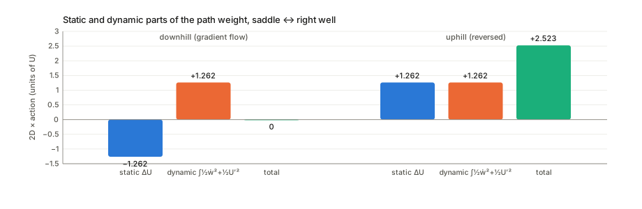
The saddle-point step of §5.2 keeps only the paths that minimise the action. The Euler–Lagrange equation of \frac12\lVert\dot w\rVert^2+V is \ddot w=\nabla V, as the paper says: Newton’s law in the upside-down potential -V. For small D, V\approx\frac12\lVert\nabla U\rVert^2, and both \dot w=-\nabla U (gradient descent) and \dot w=+\nabla U (gradient descent run backwards) solve it, since \ddot w=\mp H\dot w=H\nabla U=\nabla(\frac12\lVert\nabla U\rVert^2). Along either one, \frac12\lVert\dot w\rVert^2+\frac12\lVert\nabla U\rVert^2=\lVert\nabla U\rVert^2, whose time integral is \int\lVert\nabla U\rVert\,\lvert dw\rvert=\lvert\Delta U\rvert. So:
- downhill along gradient descent: static part \Delta U<0, dynamic part +\lvert\Delta U\rvert, total zero. Measured on the tilted double well from the saddle into the right well: -1.2616+1.2616=-2\times10^{-8};
- uphill along the reversed path: static +\Delta U, dynamic +\Delta U, total 2\Delta U, so the path weight is e^{-2\Delta U/2D}=e^{-\Delta U/D}, the Arrhenius factor. Measured: 2.5232=2\times1.2616;
- any other path costs more. The best straight constant-speed path from the left well to the saddle has total 1.6015, above the reversed gradient path’s 2\times0.7619=1.5237.
This is the Freidlin–Wentzell picture of small-noise dynamics. It has a direct consequence for the paper. Fine-tuning starts at the source solution, where the target loss is high, and goes down. On that downhill path the static factor e^{+\lvert\Delta U\rvert/2D} is larger than 1, and the reachability factor cancels it exactly. So the static factor is not a penalty in the fine-tuning direction, and the remark after eq. (15), “the transition probability is upper-bounded by a static part”, is true but vacuous exactly where the paper wants to use it.
Integrating out the valley (eqs. 11–14)
Suppose the likely path runs along a coordinate u at the bottom of a valley, and across the valley (coordinates v) the loss is quadratic with stiffness b(u):
U(u,v)=a(u)+\tfrac12\,v^\top b(u)\,v .
The particle jitters across the valley much faster than it moves along it. So at each u the v coordinates are at equilibrium, a Gaussian of covariance D\,b(u)^{-1}, and what matters for u is how much room the valley offers there. The exact bookkeeping is the marginal of the Gibbs law:
\int e^{-U(u,v)/D}\,dv=e^{-a(u)/D}\sqrt{\frac{(2\pi D)^{k-1}}{\lvert b(u)\rvert}} \qquad\Longrightarrow\qquad F(u)=a(u)+\frac D2\log\lvert b(u)\rvert+\text{const}.
F is a free energy: loss plus a penalty for narrowness. A sharp valley is a narrow corridor, and fewer noisy trajectories fit in it. The coefficient is D/2 and the sign is +. The code’s quadrature matches a+\frac D2\log b-\frac D2\log(2\pi D) to 9\times10^{-16}.
The paper arrives at U_{\text{eff}}=U+D\log\lvert H_U\rvert just before eq. (14) and in §6. In §5.2’s first paragraph and just after eq. (14) it is written with a minus sign, U-D\log\lvert H_U\rvert_{(+)}. Its eq. (13) prefactor, e^{-\frac12\log(2\pi\lvert b\rvert)}=\lvert b\rvert^{-1/2} (which also lacks a D), is folded into the static exponent \frac1{2D}U_{\text{eff}}. But the static factor is the square root of the Gibbs ratio, so a prefactor \lvert b\rvert^{-1/2} there corresponds to a Gibbs weight \lvert b\rvert^{-1}, twice the true \lvert b\rvert^{-1/2}. The correct static prefactor is \lvert b\rvert^{-1/4}.
Does the coefficient matter? It decides which minimum SGD prefers. In the code’s valley, a(u)=0.5(u^2-1)^2+0.05u makes the left well slightly deeper, and b(u)=1+99e^{-(u+1)^2/(2\cdot 0.15^2)} makes it a hundred times sharper across the valley.
| D | P(\text{sharp basin}), exact | with D\log b (paper) | with no curvature term |
|---|---|---|---|
| 0.02 | 0.938 | 0.618 | 0.993 |
| 0.05 | 0.459 | 0.104 | 0.876 |
| 0.10 | 0.294 | 0.105 | 0.721 |
| 0.15 | 0.282 | 0.145 | 0.648 |
| 0.20 | 0.289 | 0.178 | 0.609 |
A Langevin simulation at D=0.15 (2000 particles, all started in the flat well) spends a fraction 0.275 of its time in the sharp basin: the exact column, not the paper’s. The sharp, deeper basin loses its majority at D=0.046, and at D=0.179 its bottom stops being a minimum at all. There F''(-1)=4-22D changes sign, and the single sharp minimum splits into a bump with two shoulders. This is the precise content of the paper’s “sharp minima may not be minima at all” at high temperature. With the paper’s coefficient both thresholds halve (0.022 and 0.089).
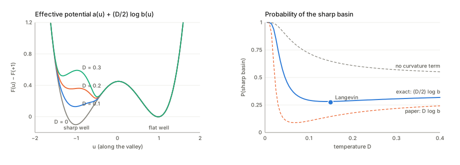
One more distinction the paper blurs. Along a path, only the transverse stiffness b(u) enters F; the curvature along the path, a''(u), does not. For the total mass of a basin, which is what a comparison of two minima needs, the Laplace approximation gives the full determinant, -D\log\int_{\text{basin}}e^{-U/D}\approx U(w^*)+\frac D2\log\lvert H_U(w^*)\rvert+\text{const}. The paper’s U+D\log\lvert H_U(w)\rvert “along the path” mixes the two.
§6 Curvature is complexity: the exact version
Why SGD’s equilibrium is the Gibbs posterior
The paper notices that with weight decay, U+D\log\lvert H_U\rvert=L+\frac\gamma2\lVert w\rVert^2+D\log\lvert\gamma I+H\rvert has the shape of eq. (4), and sets \beta=2\lambda^2\gamma. There is a cleaner statement that needs no Gaussian approximation. For any Q, completing the KL gives
\mathbb E_Q[L]+\beta\,\mathrm{KL}(Q\Vert P)=-\beta\log Z+\beta\,\mathrm{KL}(Q\Vert Q^*), \qquad Q^*(w)=\frac{P(w)\,e^{-L(w)/\beta}}{Z}.
(Expand \beta\,\mathrm{KL}(Q\Vert Q^*)=\beta\,\mathbb E_Q[\log Q-\log P+L/\beta+\log Z] and rearrange. This is the Donsker–Varadhan / Gibbs variational principle.) So the minimiser over all posteriors is the Gibbs posterior Q^*, and C_\beta^*=-\beta\log Z. With P=\mathcal N(0,\lambda^2I),
Q^*\propto\exp\Big(-\frac{L}{\beta}-\frac{\lVert w\rVert^2}{2\lambda^2}\Big), \qquad \pi_{\text{SGD}}\propto\exp\Big(-\frac{L+\frac\gamma2\lVert w\rVert^2}{D}\Big).
These are the same distribution exactly when
\beta=D\qquad\text{and}\qquad\lambda^2=\frac D\gamma .
The price of information is the SGD temperature, and the prior width is the temperature over the weight decay. Then C_\beta^*=-D\log\int e^{-U/D}dw+\text{const} is SGD’s free energy, and its Laplace approximation is the corrected eq. (4) with those values: U(w^*)+\frac D2\log\lvert H+\gamma I\rvert+\text{const}, coefficient D/2. On a 1-D double well with D=0.2 and \gamma=0.5 the code finds C_\beta(Q^*)=-\beta\log Z=0.036628. Three tilted alternatives Q_t each exceed it by exactly \beta\,\mathrm{KL}(Q_t\Vert Q^*) (0.003201, 0.000390, 0.003624). SGD’s stationary density and Q^* agree to 7\times10^{-16}.
The paper’s \beta=2\lambda^2\gamma makes the prior term \lVert w\rVert^2/2\lambda^2=\gamma\lVert w\rVert^2/\beta, so the matching Gibbs posterior is e^{-(L+\gamma\lVert w\rVert^2)/\beta}: twice the weight decay SGD actually uses, whatever \beta is. On the same example it is at total-variation distance 0.230 from SGD’s stationary law (\mathbb E w^2=0.411 under it, against 0.673 under SGD). This is the factor 2 of eq. (4) coming back. The paper also never ties \beta to D, although matching the log-determinant coefficients (\beta/2 in eq. 4, D in U_{\text{eff}}) forces it.
The upshot supports the paper’s intuition more strongly than its own derivation does. SGD at temperature D with weight decay \gamma samples the minimiser of the complexity Lagrangian with \beta=D. Raising the batch size lowers the price of information and lets SGD store more of it.
Eq. (15): which complexity, at which point?
The paper rewrites the static factor as e^{-\Delta C_\beta/2D} and reads \Delta C_\beta as “the difference in complexity between tasks”. In the path integral there is one loss, the one being trained on (the target’s, when fine-tuning), evaluated at two points. So the exponent is C_\beta^{\text{target}}(w_f)-C_\beta^{\text{target}}(w_0), the corrected target loss at the start and at the end. The static distance d_\beta=C_\beta(\mathcal D_1\cup\mathcal D_2)-C_\beta(\mathcal D_1) compares two different objectives, each at its own optimum. Those are different numbers, and the first is negative in fine-tuning (training lowers the target objective), while d_\beta is meant to be a positive cost. The step from one to the other is not made in the paper.
Eq. (16) is not Kramers’ law
Kramers’ law says a particle in a well at temperature D escapes after a time
\tau\approx\frac{2\pi}{\sqrt{U''(a)\,\lvert U''(s)\rvert}}\;e^{[U(s)-U(a)]/D},
where a is the bottom of the well and s the saddle it has to cross. The exponent is the barrier, the climb from the start to the pass. How deep the valley on the other side is does not enter: once over the pass, the particle rolls down quickly. Eq. (16), 1/\tau_K=Ce^{-\Delta C_\beta/D}, puts the difference between the two end points in the exponent instead.
The code tests this on U=h(w^2-1)^2+s(3w-w^3)/2 with h tuned so that the barrier from w=-1 is exactly 1 while the end-to-end difference \Delta U=2s runs from +0.4 to -1.5. The mean first-passage time is computed exactly from its integral formula, no simulation:
| s | \Delta U | D\ln\tau, D=0.05 | D\ln\tau, D=0.1 | d\ln\tau/d(1/D) | \tau/\tau_{\text{Kramers}} |
|---|---|---|---|---|---|
| +0.20 | +0.40 | 1.016 | 1.036 | 0.997 | 1.024 |
| 0.00 | 0.00 | 1.006 | 1.015 | 0.998 | 1.020 |
| −0.25 | −0.50 | 0.998 | 0.997 | 0.998 | 1.018 |
| −0.50 | −1.00 | 0.991 | 0.985 | 0.998 | 1.017 |
| −0.75 | −1.50 | 0.986 | 0.974 | 0.998 | 1.017 |
The slope d\ln\tau/d(1/D) is the barrier, 1, in every row. Across a change of 1.9 in \Delta U, D\ln\tau at D=0.1 moves by 0.061 (through the curvature prefactor). Eq. (16) would move it by the full 1.9.
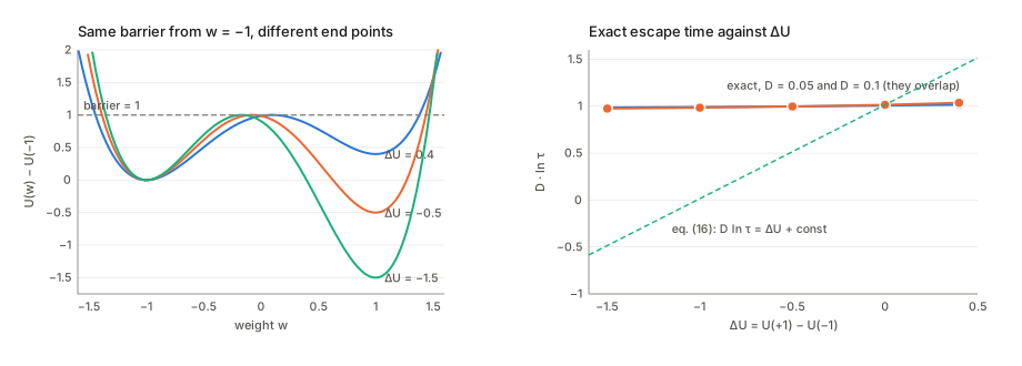
What the end-point difference does control is the ratio of forward and backward rates: k_{a\to b}/k_{b\to a}=e^{-[U(b)-U(a)]/D}. That is the detailed-balance identity above, with the full 1/D and not the 1/2D of the static factor, which explains the unexplained doubling between eq. (15) and eq. (16).
The corrected version of the paper’s idea is the multidimensional (Langer, or Eyring) rate:
\frac1\tau\approx\frac{\lvert\lambda_s\rvert}{2\pi}\sqrt{\frac{\lvert H_U(a)\rvert}{\lvert\det H_U(s)\rvert}}\;e^{-[U(s)-U(a)]/D} =\frac{\sqrt{\lvert\lambda_s\rvert}}{2\pi}\,e^{-[F(s)-F(a)]/D}, \qquad F=U+\frac D2\log\lvert H_U\rvert_+ ,
where \lambda_s is the one negative eigenvalue at the saddle and \lvert H_U\rvert_+ the product of the positive ones. This is where the paper’s “\lvert H\rvert_+” belongs: in a free-energy barrier to a saddle, with coefficient D/2. It is not a difference of task complexities, and in fine-tuning there may be no barrier at all, in which case the time is the deterministic descent time and there is no exponential.
§7 The experiments, re-read
Figure 1 (left): random labels
Time to converge grows from about 2,900 to 4,700 steps as 30,000 labels are randomised. The paper reads this as \ln\tau\propto C_\beta with C_\beta linear in the number of random labels. Over a factor of 1.6 an exponential and a straight line through the same end points differ by 2.9\% at mid-range (3,692 against 3,800 steps), so the plot cannot tell the two apart. Fig. 1 (right) fits straight lines on linear axes, i.e. \tau\propto C, not \ln\tau\propto C.
Figure 1 (right): magnitudes
The complexity axis runs to 7\times10^6 (nats, presumably). With the identification \beta=D, \Delta C_\beta/D=\Delta L/D+\Delta\mathrm{KL}, so a KL difference of 10^6 nats puts e^{-10^6} in eq. (16). The formula cannot be meant literally at these scales. What is tested is a monotone trend with fitted constants, one per architecture.
Figure 1 (centre): batch size
With D=c/B, eq. (16) gives \tau\propto e^{\Delta C_\beta B/c}. If \Delta C_\beta>0 that grows with B, the opposite of the figure. If \Delta C_\beta<0 it falls, but towards zero as B\to\infty, as if full-batch gradient descent converged in no steps. The figure (about 1,450 steps at B=100 falling to 560 at 350, then levelling) fits neither.
A mechanism that does produce that shape: the noise floor. On a quadratic loss in k dimensions SGD’s stationary loss is kD/2 (each direction holds D/2 on average, equipartition). A threshold near that floor is hit late, because only the noise’s downward excursions reach it. The code computes the exact mean time for \lvert w\rvert to bring the loss from 50 to 1.5 in k=100 dimensions with D=2/B:
| B | 70 | 80 | 100 | 150 | 200 | 300 | 400 | 1000 |
|---|---|---|---|---|---|---|---|---|
| time | 2.82 | 2.52 | 2.26 | 2.03 | 1.95 | 1.87 | 1.84 | 1.79 |
It falls steeply just above B=66.7, where the floor kD/2 equals the threshold, and levels off at the gradient-flow time \ln(10/\sqrt3)=1.753. (A direct simulation at B=70 gives 2.83.) No barrier and no task complexity is involved. Since the paper’s “converged” means “loss below a threshold”, this effect is present in its experiments too, and it is not separated from the one the paper proposes.
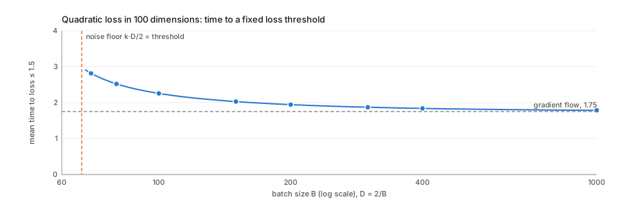
Figure 2: fine-tuning times against the static distance
The figure prints both 8\times8 matrices, so the scatter can be recomputed. Rows are the target and columns the source in both matrices: CIFAR-100 \to CIFAR-10 (row cifar10, column cifar100) takes 17.2 epochs at d=0.01, and CIFAR-10 \to CIFAR-100 takes 42.3 at d=0.52. That matches the text (“easier to go from a complex task to a related simple one”). The centre caption’s “from one task (row) to another (column)” has it the other way round. The left caption also calls its entries “the time to convergence”; they are the distances.
- Pooled, over the 48 converged pairs outside the MNIST-target row (whose times are under one epoch and off the paper’s scatter), r(d,\log_2\text{epochs})=0.64; with that row, 0.47 over 55 pairs. The fitted slope, 1.98 doublings per unit of d, reads as epochs \propto e^{d/0.73}.
- Pooling could be misleading. Targets differ in difficulty (Letters takes 53–80 epochs from anywhere, MNIST under 1), and the distance to a hard target is large from anywhere. A pooled correlation could then measure “which targets are hard”, which is §7.1’s complexity-from-scratch result again, not transfer.
- Within each target it survives. Centring both quantities per row, r=0.58 (0.61 without MNIST). The distance does rank sources for a fixed target. It is strongest for the CIFAR-100, natural and artificial targets (Spearman 0.93 each) and weakest for fashion and ifashion (0.18, 0.11). Between targets, row means correlate at 0.75.
- Direction. In 23 of the 27 pairs converged both ways, the direction with the larger distance is also the slower one.
- The one visible case of unreachability is MNIST \to Letters: no convergence, although its distance (0.68) is below that of Fashion \to Letters (0.72, converged in 79.7 epochs). That is the paper’s “nearby but unreachable” phenomenon, and the only place the data point at the dynamic factor.
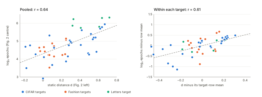
This is the best evidence in the paper, and it is better than the paper presents it. The claims about why it holds (eqs. 15–16) are what the sections above take apart.
Questions and doubts
- The abstract promises “strict lower bounds on the complexity necessary to learn a task starting from the solution to another”. No bound is stated or proved. What the text has is an approximate factorisation (eq. 10, exact) followed by saddle-point and adiabatic approximations (eqs. 11–14) and an identification (eq. 15). The one inequality mentioned, “upper-bounded by a static part”, is vacuous downhill, as shown above.
- Eq. (16) is a barrier law with the wrong exponent. Kramers’ and Langer’s rates depend on the free-energy barrier to a saddle. The difference between the two end points only fixes the ratio of forward and backward rates. The exact first-passage times above are flat in \Delta U at fixed barrier. A task-to-task version would need the barrier between the source solution and the target’s basin in the target’s loss, which neither the theory nor the experiments compute.
- Which loss? The static factor involves the loss being trained on, at two points. The static distance involves two different objectives at their own minima. The identification between them in eq. (15) is asserted, not derived. It is also sign-reversed for fine-tuning, which goes downhill.
- Constants. The curvature correction is (D/2)\log\lvert H\rvert with a + sign. The paper has +D\log\lvert H\rvert before eq. (14) and in §6, and -D\log\lvert H\rvert in §5.2’s opening and just after eq. (14). Eq. (4)’s 2\lambda^2/\beta should be \lambda^2/\beta and \Sigma^* loses its \frac12s. With those fixed, the exact identification is \beta=D, \lambda^2=D/\gamma. The printed \beta=2\lambda^2\gamma doubles the weight decay and leaves \beta unrelated to the temperature.
- The asymmetry argument. The paper motivates the whole program by transfer being asymmetric. In a fixed landscape the dynamic factor is exactly symmetric, so any asymmetry the dynamics add must come from the two tasks having different landscapes. That is a statement about U_A against U_B, which the paper’s formalism (one U at a time) does not reach.
- Negative distances and the averaged loss. With L_{\mathcal D} a mean over samples, d_\beta can be negative, and 9 of Figure 2’s 56 entries are. With a summed loss it cannot. Which normalisation the matrix uses, and whether \beta was scaled with N, is not stated. Nor is how the matrix, which spans -0.19 to 0.72, relates to Figure 1 (right)’s complexities of order 10^6.
- The noise model. Everything assumes isotropic, state-independent white noise. SGD noise is anisotropic and aligned with the Hessian (its covariance is close to the Fisher), which changes the stationary law away from Gibbs and breaks detailed balance. The paper acknowledges this in one sentence. The factorisation of eq. (10), and so the identification with C_\beta, needs it.
- Batch size. The direction of Figure 1 (centre) is not what eq. (16) predicts, whatever the sign of \Delta C_\beta, and a noise-floor effect reproduces its shape. An experiment that varied the loss threshold relative to kD/2 would separate the two.
- Small slips. Eq. (1) cancels its own noise. f=\nabla U should be -\nabla U. The Fisher expansion misses \frac12, and the KL has +\log\lvert\Sigma\rvert. Eq. (13)’s prefactor lacks D. “Kullbach-Liebler”, “Kramer’s”, “Stratonovic”. The sentence defining “the Information in the Weights” in §3 is garbled. The ELBO corresponds to \beta=1/N with an averaged loss, not \beta=1.
Takeaways
- SGD samples a Gibbs posterior, and its temperature is the price of information. With weight decay \gamma and noise level D\propto\eta/B, the stationary law minimises \mathbb E_Q[L]+\beta\,\mathrm{KL}(Q\Vert P) exactly, for \beta=D and prior variance D/\gamma. That is the solid core of the paper’s link between dynamics and task complexity.
- Static times reachability is detailed balance. The end-point factor is \sqrt{\pi(w_f)/\pi(w_0)}. The path factor is symmetric and carries all the time dependence, so “is there a road” is the whole question and “how far down is the destination” only sets the forward/backward ratio.
- Downhill is free, uphill costs \Delta U/D. On the most likely paths the static and dynamic parts cancel going down and add going up. Waiting times are set by barriers, not by end points.
- Flat minima win by \frac D2\log\lvert H\rvert. Integrating out the directions across a valley adds half D times the log-determinant of the transverse curvature. At a high enough temperature a sharp minimum becomes a bump, the precise form of “sharp minima may not be minima”.
- The static distance does predict fine-tuning cost, within a target. Re-read from its printed numbers, Figure 2 supports the distance as a ranking of sources (r\approx0.6 within target rows, 23 of 27 directions right). That is more than the pooled scatter shows, and more than the theory derived for it.