Features are fate: a theory of transfer learning in high-dimensional regression
Links
- arXiv:2410.08194:
the preprint (v2, July 2025, is the ICML version). Authors’ code: javantahir/features_are_fate.
In the part of the repository I could read (a summary of
plots.ipynb) I found the phase-diagram code but not the code for Figure 3(d) or Figure 4, so those two are reproduced here from the text, not compared with their scripts. - Interactive
companion: seven widgets. (1) Eq. (11) as a phase diagram
you can click. (2) Scratch risk against the flat linear-transfer floor.
(3) Eq. (15) and the null-space geometry.
- The ridge result and the finite-n dip. (5) KL against transferability for \theta\in[0,\pi]. (6) The Dudley metric saturating, and the failing proof line. (7) A finite-sample Wasserstein estimate that measures dimension, not tasks.
- Runnable checks, in
code/:theory.py(every closed form in one place),transfer_theory.py(Monte Carlo, real gradient descent on two-layer linear networks, the algebra of Sections 3 and C),appendix_a.py(Appendix A and Figure 4),relu_projection.py(Figure 3d). Every number below comes from one of them.make verifyruns all four. - Integral probability metrics: the page Integral probability metrics: a panel of judges answers “what is a Dudley metric, what is an IPM” from scratch with its own interactive widgets. The short version is in the first question below.
- Background pages this one leans on: the four fundamental subspaces (row space, null space, the pseudo-inverse and why gradient descent from zero finds the minimum-norm solution) and optimal transport (the Wasserstein distance).
- Other transferability notes in this collection that this paper’s picture speaks to: Achille 2019, task reachability (a fine-tuning success also depends on the starting weights), Nguyen 2020, LEEP, You 2021, LogME, Bao 2019, H-score, Chaves 2023 and Claßen 2026 (the scores fail on medical tasks), Jacot 2018, NTK and Fort 2020 (the lazy regime that the paper’s tiny-initialisation limit is the opposite of).
Javan Tahir, Surya Ganguli and Grant Rotskoff, Features are fate: a theory of transfer learning in high-dimensional regression, ICML 2025. Stanford University, Applied Physics and Chemistry.
In one paragraph
When does starting from a pretrained network beat training from scratch on a small target set? The paper answers this in a model where every quantity has a formula: a deep linear network trained by gradient flow from a tiny initialisation, Gaussian inputs, a linear target function and label noise. Pretraining on an unlimited source set leaves the hidden layer holding one direction, \beta_s, the source’s weight vector. After that the story is a comparison of two closed-form risks. Scratch training is minimum-norm least squares and follows a double-descent curve in \gamma=n/d. Transfer can only re-scale \beta_s, so it has a floor \sin^2\theta (the target’s part orthogonal to the source direction) that no amount of target data lowers. Their difference \mathcal T is the transferability, and it is positive for few samples and small angle, negative for many samples or a wide angle, and positive again in a thin band around \gamma=1 where scratch training is at its worst. Fine-tuning keeps the pretrained network’s guess in the directions the data cannot see, so it beats scratch exactly when the source vector is closer to the target than the origin is: \theta<60^\circ. Appendix A argues that distances between the two data distributions (Dudley, Wasserstein-1, KL) cannot predict any of this because two tasks in the same feature space can be arbitrarily far apart, and a short numerical section checks that the picture survives with ReLU networks. I re-derived and simulated every formula: they are right. The places where I disagree are the proof of Theorem A.2 (a step fails and the statement needs “any \delta<2” for Dudley), the exactness of Theorem 3.9 (a scale factor c=1+O(\sigma^2) is missing, small at the paper’s \sigma=0.2 and large at \sigma=1), and Figure 4(b), whose Wasserstein axis measures sampling noise.
The spine of the argument
- Setting. y=\beta^\top x+\epsilon, x\sim\mathcal N(0,I_d), \lVert\beta_s\rVert=\lVert\beta_t\rVert=1, \beta_s^\top\beta_t=\cos\theta, noise \sigma. Scratch and transfer see the same n=\gamma d target points. \mathcal T=\mathbb E[R_{sc}-R_{tx}].
- Pretraining sparsifies the features (Lemma 3.3, Theorem 3.4). A two-layer linear net started at scale \alpha\to0 has a conserved quantity that makes its layers balanced, so the hidden layer becomes rank one and aligned with \beta_s.
- Scratch training is minimum-norm interpolation (Theorem 3.5), whose risk is the double-descent curve (Theorem 3.6, eq. 8).
- Linear transfer regresses the target onto the one scalar feature \beta_s^\top x (Theorem 3.7, eq. 10): risk \sin^2\theta+O(1/n). So \mathcal T_{lt}=R_{sc}-\sin^2\theta (eq. 11), a phase diagram in (\theta,\gamma) with three regions.
- Ridge does not help (Theorem 3.8, eq. 13): it only shrinks the one coefficient.
- Fine-tuning moves only the part of the solution the data can see and leaves the rest at the pretrained guess (Theorem 3.9, eq. 15): \mathcal T_{ft}=(1-\gamma)(2\cos\theta-1) for \gamma\le1, and 0 beyond.
- A ReLU student–teacher model shows the same shape, with the feature space replaced by an RKHS (Section 4).
- Appendix A: distribution-level distances do not track any of this.
Setup and notation
| Symbol | Meaning |
|---|---|
| d,\;n,\;\gamma=n/d | input dimension, target sample size, and their ratio; the limit n,d\to\infty with \gamma fixed |
| \beta_s,\;\beta_t\in\mathbb R^d | unit weight vectors of the source and target linear functions; \cos\theta=\beta_s^\top\beta_t |
| \sigma | label-noise standard deviation; the SNR of the target is 1/\sigma^2 |
| X\in\mathbb R^{n\times d}, y | target design matrix (i.i.d. Gaussian rows) and labels y=X\beta_t+\epsilon |
| X^+, P=X^+X | pseudo-inverse and the orthogonal projector onto the row space of X (a random \min(n,d)-dimensional subspace of \mathbb R^d) |
| W_1,\dots,W_L, \alpha | weights of the deep linear network f(x)=x^\top W_1\cdots W_L and the initial scale W_l(0)=\alpha\bar W_l; \alpha\to0 is the “rich” or feature-learning regime |
| \beta(t)=W_1\cdots W_L | the end-to-end linear map; gradient flow moves it inside the loss landscape of the network |
| R=\mathbb E_x(f(x)-f^*(x))^2=\lVert\hat\beta-\beta_t\rVert^2 | generalisation error (risk) with noise-free targets |
| R_{sc},\;R_{lt},\;R_{ft} | risk of scratch training, linear transfer (last layer only) and fine-tuning (everything) |
| \mathcal T=\mathbb E_{\mathcal D}(R_{sc}-R_{tx}) | transferability: positive means the pretrained start wins |
| z=X\beta_s,\;w=X\nu | the projections of the data onto the source direction and onto the part of \beta_t orthogonal to it; independent \mathcal N(0,I_n) vectors |
| D_l=W_l^\top W_l-W_{l+1}W_{l+1}^\top | the conserved “balancedness” of adjacent layers under gradient flow |
Two conventions in the paper are worth stating once. Gradient flow is the continuous-time limit of gradient descent, with the learning rate set to 1 for analysis. The order of limits is \lim_{\alpha\to0}\lim_{t\to\infty}: at each fixed \alpha train until the loss has converged, then shrink the initial scale.
Questions from a first reading
Six questions from a first pass through the paper, in the order they were asked. Each answer starts with the idea in plain words, then gives the formula, then a number from the code. The sections after this one go through the paper in its own order.
What is a Dudley metric? What is an IPM (integral probability metric)?
Plain version. To say how far apart two distributions P and Q are, hire a judge: a function h that gives every outcome a score. Average the score over draws from P, do the same for Q, and look at the gap. One judge gives one gap. An integral probability metric is the gap of the best judge in a fixed panel \mathcal F:
\gamma_{\mathcal F}(P,Q)\;=\;\sup_{h\in\mathcal F}\;\bigl\lvert\,\mathbb E_{x\sim P}\,h(x)\;-\;\mathbb E_{x\sim Q}\,h(x)\,\bigr\rvert .
Read \mathbb E_{x\sim P}h(x) as “the average of h over data drawn from P”: for a data set it is the sample mean of h over its points, for a density p it is \int h(x)p(x)\,dx. The whole content of a metric is the choice of panel. Judges scoring in [0,1] give total variation. Judges that may not slope steeper than 1 give the Wasserstein-1 (earth mover’s) distance (Kantorovich–Rubinstein duality; see optimal transport). The unit ball of a kernel’s function space gives MMD (and HSIC is an MMD between a joint law and the product of its marginals).
The Dudley metric (also called the bounded-Lipschitz metric) uses judges with a budget: their height plus their steepness may not exceed 1,
\gamma_\beta(P,Q)=\sup_{\lVert h\rVert_{BL}\le1}\bigl\lvert\mathbb E_Ph-\mathbb E_Qh\bigr\rvert,\qquad \lVert h\rVert_{BL}=\underbrace{\lVert h\rVert_L}_{\text{steepest slope}}+\underbrace{\lVert h\rVert_\infty}_{\text{largest score}} .
A tall judge must be flat and a steep judge must be short. That is what makes it behave differently from its neighbours. Two point masses at 0 and D (two clusters of embeddings a distance D apart) show it in closed form: TV is 1 for every D>0 (the supports are disjoint, TV saturates immediately), W_1=D (grows without limit), and Dudley is 2D/(D+2): it grows like D for small D and saturates at 2 for large D. (Derivation: a judge with height a and slope 1-a can separate the two points by \min(2a,(1-a)D); equalising gives a=D/(D+2).) Three facts follow from the panel being small: \gamma_\beta\le W_1 (its judges are inside the 1-Lipschitz ball), \gamma_\beta\le 2\,\mathrm{TV}\le2 (every score is at most 1), and it metrizes weak convergence (a standard fact that I have not re-derived). The foundations page has an interactive that draws these judges for two densities and plots all four distances (and KL) against the separation. One caution from that page: “Dudley behaves like W_1 for nearby distributions” holds only for distributions narrow compared with the unit scale: for two unit-width Gaussians the ratio of Dudley to W_1 tends to 0.35 as the shift goes to 0, not 1. Its numbers for \mathcal N(0,1) against \mathcal N(1,1) are TV =0.383, Dudley =0.343, W_1=1, KL =0.5.
KL and friends are a different family. \varphi-divergences such as KL compare the two probability tables point by point, need P to be absolutely continuous with respect to Q, and are infinite (or saturated) when the supports do not overlap. IPMs need a notion of distance on the sample space (for smooth judges) and stay finite. Total variation is the only member of both families. The paper cites Sriperumbudur et al. (2009) for the framework and uses it for one purpose, in Appendix A, discussed next.
Help me understand Appendix A. How does it show that dataset similarity is not predictive of transfer efficiency?
The claim in plain words. “Similar tasks transfer well” sounds obvious, so the appendix asks what “similar” could mean if it is measured on the data: how far apart the joint laws p_s(x,y) and p_t(x,y) are, in Dudley distance, Wasserstein-1 or KL. The paper’s answer is that this cannot be the right notion, because two target functions can lie in the same feature space (so that a pretrained network transfers to either by re-learning a few output weights) while their data distributions are arbitrarily far apart.
Setting. A feature space \Phi\subset L_2(p) is a linear span of orthonormal functions \phi_1,\dots,\phi_M. For f\in\Phi, the data law is p_f(x,y)=p(x)\,\mathcal N(y;f(x),\sigma^2): draw x, then a noisy label around f(x). Note that this needs \sigma>0: with no noise p_f lives on the graph of f and has no density.
Theorem A.2. For every f\in\Phi and every \delta>0 there is a g\in\Phi with \gamma_\beta(p_f,p_g)\ge\delta and, separately, one with D_{KL}(p_f\Vert p_g)\ge\delta.
How the logic is meant to go. (i) Theorem A.2: within one feature space, distribution distances can be made as large as you like. (ii) Section 3: for targets in the same feature space (they take \theta=0) transfer is positive, because only output weights need re-learning. (iii) So large distance does not mean poor transfer, and a distance between datasets cannot be the predictor.
The KL half, line by line. With y\mid x\sim\mathcal N(f(x),\sigma^2) the KL between the two conditional laws is (f(x)-g(x))^2/(2\sigma^2), and averaging over x gives (eqs. 32–35)
D_{KL}(p_f\Vert p_g)=\frac{\lVert f-g\rVert_{L_2(p)}^2}{2\sigma^2}.
The code confirms it by quadrature (for f=x, g=-x, \sigma=0.2: 50.0000 both ways). This is right and unbounded, so taking g=-\alpha f with large \alpha works. One slip: the paper takes \alpha>\sigma\sqrt\delta/\lVert f\rVert, which only gives D_{KL}>\delta/2 (since (1+\alpha)^2\ge\alpha^2 and \alpha^2\lVert f\rVert^2/(2\sigma^2)>\delta/2). For \lVert f\rVert=0.01, \sigma=0.2, \delta=100 that choice gives D_{KL}=50.5<\delta. The fix is \alpha>\sigma\sqrt{2\delta}/\lVert f\rVert: harmless.
The Dudley half, line by line. The proof (Appendix D.1) picks one judge, h(x,y)=\tfrac12\cos y. Its steepest slope is \tfrac12 and its largest score is \tfrac12, so \lVert h\rVert_{BL}=1: it is in the panel. That is a legitimate way to lower-bound a supremum: exhibit one judge. Since \mathbb E\cos y=e^{-\sigma^2/2}\cos f(x) when y\sim\mathcal N(f(x),\sigma^2),
\gamma_\beta(p_f,p_g)\;\ge\;\frac{e^{-\sigma^2/2}}{2}\,\Bigl\lvert\int\bigl[\cos f(x)-\cos g(x)\bigr]p(x)\,dx\Bigr\rvert\qquad\text{(line 28)}.
The next line (29) claims this is at least \tfrac{e^{-\sigma^2/2}}{2}\int[f(x)^2+g(x)^2]p(x)\,dx,
“by the identity \cos x+x^2\ge\cos
z-z^2”. This step is wrong. (a) The left side is
at most e^{-\sigma^2/2} whatever g is (\lvert\cos
f-\cos g\rvert\le2), while the right side grows without bound as
g grows. (b) It even fails for g=f: the left side is 0 and the right side is e^{-\sigma^2/2}\lVert f\rVert^2>0. (c) The
identity is true but rearranges to \cos x-\cos
z\ge-(x^2+z^2), a lower bound by a negative number,
which says nothing about the absolute value. Numbers for f=x, x\sim\mathcal
N(0,1), \sigma=0.2
(appendix_a.py):
| g | line (28) | line (29) right side |
|---|---|---|
| x | 0.0000 | 0.9802 |
| 3x | 0.2918 | 4.9010 |
| 10x | 0.2973 | 49.5000 |
The last row of line (28) is also the best this judge can ever do against g=cx: 0.2973.
And the theorem as stated cannot be true for large \delta. Every judge in the panel has \lvert h\rvert\le1, so \gamma_\beta\le2 for any two distributions. “For every \delta>0” fails for \delta\ge2. The honest reading is “as far as the metric permits”. A judge that shows this: for g=cf use h(y)=a\bigl(1-2\min(\lvert y\rvert/K,1)\bigr) with a=K/(K+2), which has height a and slope 2a/K so \lVert h\rVert_{BL}=1. It gives, for f(x)=x and \sigma=0.2:
| c | 2 | 10 | 100 | 1000 | 10^5 |
|---|---|---|---|---|---|
| Dudley \ge | 0.27 | 0.96 | 1.61 | 1.87 | 1.99 |
| KL | 12.5 | 1012 | 1.2\times10^5 | 1.2\times10^7 | 1.25\times10^{11} |
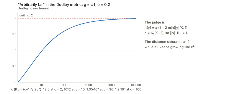
The paper’s remark that the result “also holds for any IPM over a larger function class, in particular W_1” is correct (a bigger panel has a bigger supremum), and for W_1 and KL “arbitrarily far” is literal. The conclusion survives; the proof as printed does not.
Does it apply to the phase diagrams? Only after one more step. The construction uses g=cf with large c, so \lVert g\rVert=c\ne1, outside the unit-norm family of Assumption 3.2. The transfer analysis extends trivially: for a target c\beta_s scratch training has risk c^2(1-\gamma)+\gamma\sigma^2/(1-\gamma) while linear transfer has risk \sigma^2/(n-2), so \mathcal T\approx c^2(1-\gamma)+\dots grows with the distance. Monte Carlo at d=200, \gamma=0.5, \sigma=0.2 gives \mathcal T=0.54,\,2.02,\,4.58,\,50.2 for c=1,2,3,10 (formula 0.54,\,2.04,\,4.54,\,50.0). So Theorem A.2 plus Section 3 does establish “large distance, positive transfer”. That is sufficiency-failure: distance being large does not imply poor transfer. It does not establish the other direction (small distance, poor transfer), and “not predictive” needs both.
A cleaner argument the paper does not make: same pair of tasks, many sample sizes. \mathcal T depends on n, and a distance between p_s and p_t does not. Fix \theta=\pi/4 and \sigma=0.2. The pair has one KL, (1-\cos\theta)/\sigma^2=7.32, and one Dudley or W_1 distance. Yet eq. (11) gives \mathcal T_{lt}>0 for \gamma<0.549, <0 on (0.549,0.911), >0 on (0.911,1.080) and <0 beyond 1.080. Any function of (p_s,p_t) alone is constant along that path, so it cannot determine the sign of \mathcal T. This is the real reason a dataset distance fails: transferability is a property of the pair and the amount of target data and noise, through the feature space.
Figure 4 reproduced. The paper’s Figure 4 sweeps \theta and plots \mathcal T against KL (a) and against a finite-sample W_1 (b). Two things I found:
- (a) is a sweep of \theta over [0,\pi], not [0,\pi/2]. Within the paper’s family D_{KL}(p_s\Vert p_t)=\lVert\beta_s-\beta_t\rVert^2/(2\sigma^2)=(1-\cos\theta)/\sigma^2, which reaches 2/\sigma^2=50 at \theta=\pi for \sigma=0.2: exactly the axis of Figure 4(a). \mathcal T_{lt} depends on \theta only through \sin^2\theta, which is symmetric about \pi/2, so it goes down and comes back up. At \gamma=0.5, \sigma=0.2: \mathcal T=+0.540 at \theta=0, -0.460 at \pi/2, +0.540 at \pi (Figure 4a reads about +0.54,-0.46,+0.54). The target \beta_t=-\beta_s is as far as it gets in KL and transfers exactly as well as \theta=0, because linear transfer just flips the sign of one coefficient. Over [0,\pi] the correlation between KL and \mathcal T is -0.000. Over the paper’s phase-diagram range [0,\pi/2] it is -0.972 and the rank correlation is exactly -1: inside the range the paper draws, KL orders \mathcal T_{lt} perfectly at fixed (\gamma,\sigma). The text never says the sweep extends past \pi/2.
- (b) is sampling noise. The W_1 axis of Figure 4(b) spans 526 to 529 and the scatter has no shape. Population W_1 between p_s and p_t is at most \sqrt{2/\pi}\,\lVert\beta_s-\beta_t\rVert\le1.60 (couple the same x and the same noise; then \lvert y_s-y_t\rvert=\lvert(\beta_s-\beta_t)^\top x\rvert). But two independent samples of \mathcal N(0,I_{500}) are far apart in the sample space and an exact optimal-transport solver sees it. With \gamma=0.5 (n=250), d=500, \sigma=0.2 and an \ell_1 ground metric I get W_1=526.3 at \theta=0 (identical laws), 527.5 at \pi/2 and 527.6 at \pi; with \ell_2, 29.7 at all three. The \ell_1 value matches the paper’s axis, which suggests (I could not confirm; their Figure 4 code is not in the released repository) that this is what was plotted. In d=2 the same estimator is informative and rises monotonically with \theta, like KL. So Figure 4(b) shows a property of the estimator in 500 dimensions, not of the population distance.
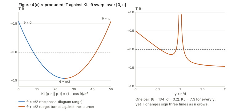
Summary of what Appendix A does and does not show. It shows that a large dataset distance is compatible with excellent transfer (once the norm restriction is lifted, and with “large” read as “near the metric’s ceiling” for Dudley). With my additions it shows that no function of the pair (p_s,p_t) can determine the sign of \mathcal T. It does not show, and the paper’s Figure 4 does not show, that distances are uncorrelated with transferability within the paper’s own family and range.
Why assume label noise?
Four separate reasons, in order of importance.
- Without noise there is nothing for transfer to win. Scratch training is exact once n>d: with \sigma=0 the risk (8) is 0 for \gamma>1, and \mathcal T_{lt}=-\sin^2\theta<0 at every \theta>0. The noiseless diagram (Figure 7) is red everywhere above \gamma=1; below \gamma=1 the sign is that of (1-\gamma)-\sin^2\theta, so transfer wins exactly for \gamma<\cos^2\theta. Noise is what makes the large-n half of the diagram interesting: with noise scratch training pays a variance term \sigma^2/(\gamma-1) for estimating d coefficients from noisy labels, while transfer estimates one coefficient and pays only \sigma^2/(n-2). That variance gap is the whole reason transfer can win with plenty of data.
- It creates the double-descent spike. The blow-up of R_{sc} at \gamma=1 comes from amplifying noise through the smallest singular value of X; with \sigma=0 there is no spike and no anomalous-positive-transfer band.
- It makes Appendix A well posed. p_f(x,y)=p(x)\mathcal N(y;f(x),\sigma^2) has a density only for \sigma>0, and D_{KL}=\lVert f-g\rVert^2/(2\sigma^2) is finite only then (and is inversely proportional to \sigma^2: the smaller the noise the “farther apart” the same two functions look).
- It is realistic, and it sets the interesting scale: the target’s signal-to-noise ratio is 1/\sigma^2. Negative transfer for \gamma<1 needs \sigma<1 (SNR above 1) and, more precisely, \theta>\arccos(1-\sigma) (36.9^\circ for \sigma=0.2; for \sigma\ge1 negative transfer at \gamma<1 disappears at every \theta\le\pi/2).
Figure 1 seems to suggest that they are working on a toy linear regression model and not deep learning
Correct, and the paper says so in its own words: “deep linear networks” in the abstract and a “limited to affine transformations” caveat in Section 3. The function class is linear, f(x)=\beta^\top x, the target is linear and the data are Gaussian. What is deep about it is the training dynamics: the network is parameterised as W_1\cdots W_L, and gradient flow on that product has an implicit bias (towards minimum norm, and towards rank-one hidden layers from a small start) that gradient flow on \beta directly would not have. Depth does not change what the network can represent. Two ways to read this.
- What the model buys. A closed form for a phenomenon that is otherwise only seen empirically: the pretrained network keeps exactly one direction, so “the feature space” is a definite object. In a real network the feature space is what the last hidden layer spans and is never cleanly identifiable, which is why the paper retreats to a solvable case.
- What it costs. With a one-dimensional feature space the floor \sin^2\theta is a sharp cliff. A network with k features has floor \rho=\lVert P_\perp\beta_t\rVert^2 (the part of the target outside the feature span) and, by the same proof, risk \rho+(\sigma^2+\rho)\,k/(n-k-1); I checked this for k=1,5,20 (for k=5, n=120, \rho=0.2: MC 0.2134\pm0.0004, formula 0.2127). That is my extension, not the paper’s.
The ReLU section (Section 4) is the bridge to a nonlinear model: a two-layer student–teacher net with m=1000 hidden ReLU units against a teacher with m_*=100, d=100. The paper claims a qualitatively identical picture. It is supported less strongly: there is no formula for the scratch risk, so the negative transfer boundary is found by equating the empirical power law R_{sc}\approx An^{-1.18} with the estimated out-of-RKHS norm. See the doubts below. It is also still a teacher–student setup with random Gaussian data, far from ImageNet-scale deep learning.
Figure 1 suggests that increasing target dataset size hurts the transfer score, and the same for task overlap. Seems counterintuitive
Two separate points.
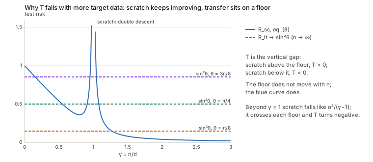
Target set size. More data does not hurt transfer. It helps both models, but scratch training improves faster and the score is their difference. Look at eq. (10) and eq. (8) side by side:
- Linear transfer has risk \sin^2\theta+(\sigma^2+\sin^2\theta)/(n-2). It is close to its floor \sin^2\theta already at small n and cannot go below it: the network can only express the one direction \beta_s, so the part of the target orthogonal to it is invisible however much data you add.
- Scratch training has risk \sigma^2/(\gamma-1) beyond \gamma=1, which keeps falling towards 0: it can express every direction.
So \mathcal T=R_{sc}-\text{floor} starts high (scratch has almost nothing at small n: the risk is 1 at \gamma\to0, the risk of predicting zero), falls as scratch catches up, spikes at \gamma=1 where scratch is at its worst, and settles at -\sin^2\theta (plus \sigma^2/(\gamma-1)). At \theta=\pi/4, \sigma=0.2: \mathcal T_{lt}=+0.263,\,+0.040,\,-0.130,\,-0.460 at \gamma=0.25,\,0.5,\,0.75,\,2. This is the familiar rule that pretraining helps most when target data are scarce. The figure below shows it as a moving curve against a fixed line.
Task overlap. The horizontal axis of Figure 1 is the angle \theta, not the overlap. A larger \theta is less overlap (\cos\theta is the overlap). \mathcal T_{lt} falling with \theta is therefore “less similar tasks transfer less”, which is the intuitive direction: scratch training does not depend on the source at all, and the floor \sin^2\theta grows with \theta. The one non-obvious feature in the angle direction is the band at \gamma\approx1, which stays blue even at \theta=\pi/2 (orthogonal tasks), the paper’s “anomalous positive transfer” (the risk of scratch training there exceeds 1, the risk of predicting zero: R_{sc}(0.99)=3.97).
Also note what \mathcal T is not: it is an outcome (a difference in test risk between two trainings), not a transferability estimator that one could compute from data before training, such as LEEP or LogME.
Help me understand eqs. 11 and 15. Plot these equations
Both are differences of two risks computed exactly, so I derive each risk first.
Eq. (11): linear transfer
\mathcal T_{lt}=\begin{cases}\dfrac{(1-\gamma)^2+\gamma\sigma^2}{1-\gamma}-\sin^2\theta & \gamma<1\\[2ex]\dfrac{\sigma^2}{\gamma-1}-\sin^2\theta & \gamma>1\end{cases}
The first term is scratch training (eq. 8). Gradient flow from a tiny start on the scratch network finds the minimum-norm interpolator \hat\beta=X^+y=P\beta_t+X^+\epsilon (Theorem 3.5). Split its error into what the data cannot see and what noise adds:
\lVert\hat\beta-\beta_t\rVert^2=\underbrace{\lVert(I-P)\beta_t\rVert^2}_{\text{bias: the part of }\beta_t\text{ outside the row space}}+\underbrace{\lVert X^+\epsilon\rVert^2}_{\text{variance}}
(the two pieces are orthogonal). The row space is a uniformly random n-dimensional subspace, so a fixed unit vector keeps a fraction n/d=\gamma of its squared length in it: bias =1-\gamma (and 0 for \gamma\ge1, where P=I). The noise term is \sigma^2\operatorname{tr}\bigl((XX^\top)^{-1}\bigr) and for Gaussian X the mean inverse Wishart matrix gives exactly \sigma^2 n/(d-n-1)\to\sigma^2\gamma/(1-\gamma) (and \sigma^2/(\gamma-1) for \gamma>1). Sum: (1-\gamma)+\sigma^2\gamma/(1-\gamma)=\frac{(1-\gamma)^2+\gamma\sigma^2}{1-\gamma}. The blow-up at \gamma=1 is X having a near-zero singular value there. The code checks the exact finite-size versions (1-n/d+\sigma^2n/(d-n-1) etc.) to Monte Carlo accuracy at d=200: for \gamma=0.5: 0.544 simulated, 0.540 exact; the paper’s Theorem 3.6 proof reaches the same numbers through Stieltjes transforms of the Marchenko–Pastur law.
The second term is linear transfer. The pretrained hidden layer is W_1=\beta_sv^\top (Theorem 3.4), so the features of the target inputs are the single scalar z_i=x_i^\top\beta_s, and the last layer fits one number b. Write \beta_t=\cos\theta\,\beta_s+\sin\theta\,\nu with \nu\perp\beta_s. Then, with z=X\beta_s and w=X\nu independent \mathcal N(0,I_n) vectors (rotation invariance of the Gaussian),
y=\cos\theta\,z+\underbrace{\sin\theta\,w+\epsilon}_{\text{looks like noise of variance }\sin^2\theta+\sigma^2},\qquad b=\frac{z^\top y}{\lVert z\rVert^2}=\cos\theta+\frac{z^\top(\sin\theta\,w+\epsilon)}{\lVert z\rVert^2}.
Given z, the second term is \mathcal N\bigl(0,(\sin^2\theta+\sigma^2)/\lVert z\rVert^2\bigr). The risk is \lVert b\beta_s-\beta_t\rVert^2=(b-\cos\theta)^2+\sin^2\theta, and \mathbb E[1/\lVert z\rVert^2]=1/(n-2) (the mean of an inverse chi-square with n degrees of freedom; the paper gets it from a Gamma integral, eqs. 117–121):
\mathbb E\,R_{lt}=\sin^2\theta+\frac{\sigma^2+\sin^2\theta}{n-2}\qquad\text{(eq. 10, exact for every }n>2\text{)}.
The picture to keep: the part of the target outside the source direction does two things. It sets an irreducible error \sin^2\theta, and it acts as extra label noise of the same size. Taking n\to\infty leaves \sin^2\theta, and subtracting from R_{sc} gives eq. (11). The Monte Carlo at d=200 (\gamma=0.5, \theta=\pi/8): \mathcal T_{lt}=+0.396 simulated, +0.392 from the exact formulas, +0.394 from eq. (11); real gradient descent on two-layer networks at d=20 reproduces eq. (10) too (below).
Reading the plot. The picture is: scratch risk minus a fixed floor.
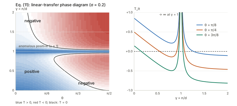
The three zero contours are exact. For \gamma>1, \mathcal T_{lt}<0 iff \gamma>1+\sigma^2/\sin^2\theta (at 45^\circ, \sigma=0.2: \gamma>1.080). For \gamma<1, \mathcal T_{lt}<0 iff \bigl(1-\gamma\bigr)^2+\gamma\sigma^2<\sin^2\theta\,(1-\gamma), which rearranges to a quadratic,
\gamma^2-\bigl(1+\cos^2\theta-\sigma^2\bigr)\gamma+\cos^2\theta<0,\qquad \gamma_\pm=\tfrac12\Bigl[\bigl(1+\cos^2\theta-\sigma^2\bigr)\pm\sqrt{\bigl(1+\cos^2\theta-\sigma^2\bigr)^2-4\cos^2\theta}\Bigr].
So negative transfer occupies \gamma\in(\gamma_-,\gamma_+) (the paper prints the interval as (\gamma_+,\gamma_-), a typo), which is non-empty iff 1-\cos\theta>\sigma, i.e. \theta>\arccos(1-\sigma). For \sigma=0.2: 36.9^\circ; at 45^\circ the interval is (0.549,0.911); at 60^\circ, (0.264,0.946); at 90^\circ, (0,0.960). As \sigma\to0 the roots tend to \cos^2\theta and 1. The code checks these against brute-force root finding on eq. (11). The thin blue band at \gamma=1 is the region where scratch training’s double-descent spike exceeds the floor: at \theta=\pi/2, \mathcal T_{lt}>0 only for \gamma\in(0.96,1.04).
Eq. (15): fine-tuning
\mathcal T_{ft}=\begin{cases}(1-\gamma)\,(2\cos\theta-1)&\gamma\le1\\0&\gamma>1\end{cases}
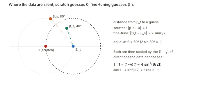
Fine-tuning trains all the weights on the target, starting from the pretrained network. The key fact is that gradient flow only ever moves the network’s end-to-end vector \beta along directions in the row space of X: the gradient of the loss with respect to \beta is X^\top(X\beta-y)/n, a combination of the rows of X. In the (1-\gamma) fraction of directions the data never touch (the null space of X), whatever the network started with is what it keeps. Start-from-scratch networks keep 0 there (the tiny initialisation); the pretrained network keeps \beta_s’s component there. In the row space both converge to the same thing, the minimum-norm interpolator \beta_{sc}. So
- scratch leaves (I-P)\beta_t as error in the null space, of squared length (1-\gamma);
- fine-tuning leaves (I-P)(\beta_t-\beta_s), of squared length (1-\gamma)\lVert\beta_t-\beta_s\rVert^2=(1-\gamma)(2-2\cos\theta).
The difference of the two is (1-\gamma)(1-(2-2\cos\theta))=(1-\gamma)(2\cos\theta-1): eq. (15). (The paper gets there by expanding a longer expression in Appendix D.8; the null-space reading is the same computation.) The picture is the distance from \beta_t to a guess: scratch guesses the origin, at distance 1; fine-tuning guesses \beta_s, at distance 2\sin(\theta/2); these are equal when \theta=60^\circ. For \gamma>1 the row space is everything, the loss has a unique minimum, gradient flow converges to it from any start, and the network forgets where it began: \mathcal T_{ft}=0.
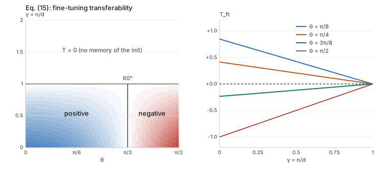
Numbers (transfer_theory.py): \mathcal
T_{ft}(\gamma=0)=+0.848,\,+0.414,\,-0.235 for \theta=\pi/8,\pi/4,3\pi/8; at \gamma=0.5: +0.424,\,+0.207,\,-0.117. Monte Carlo at
d=200 reproduces them: +0.429 vs +0.424 (\gamma=0.5, \theta=\pi/8), -0.503 vs -0.500 (\theta=\pi/2).
A correction I found to eq. (15): the null-space part carries a scale factor c. Real gradient descent does not land exactly on \beta_{sc}+(I-P)\beta_s (Theorem 3.9). For a two-layer net the pretrained state is W_1=\beta_sv^\top, W_2=v with \lVert v\rVert=1 and the layers balanced (\lVert W_1\rVert=\lVert W_2\rVert, from the conserved quantity D_1\approx0). During fine-tuning the updates \dot W_1=-rW_2^\top, \dot W_2=-W_1^\top r (with r=\nabla_\beta L\in\operatorname{row}(X)) keep W_1=u\,v^\top and W_2=c\,v with v fixed, the null-space part of u fixed at (I-P)\beta_s, and \beta=c\,u. Interpolation forces the row-space part of \beta to equal \beta_{sc}, and balancedness \lVert u\rVert^2=c^2 (conserved) fixes the scale:
\beta_{ft}=\beta_{sc}+c\,(I-P)\beta_s,\qquad c^4-a\,c^2-b=0,\quad a=\lVert(I-P)\beta_s\rVert^2\to1-\gamma,\; b=\lVert\beta_{sc}\rVert^2\to\gamma+\frac{\sigma^2\gamma}{1-\gamma}.
The paper’s version is c=1, which holds iff a+b=1, i.e. iff \sigma=0 (at large d). Redoing the risk with c: R_{ft}-R_{sc}=(1-\gamma)(c^2-2c\cos\theta), so \mathcal T_{ft}=(1-\gamma)(2c\cos\theta-c^2) with break-even \cos\theta=c/2. At the paper’s \sigma=0.2 the correction is invisible (c=1.005 at \gamma=0.25, break-even 59.8^\circ). It is not small at higher noise: at \gamma=0.5, \sigma=1, c=1.225, break-even 52.2^\circ, and eq. (15) predicts \mathcal T_{ft}=0 at 60^\circ where the truth is about -0.13. Evidence, all from the code: real gradient descent on two-layer networks at d=20 with a small enough step (gradient descent with step 0.1 drifts off the conserved quantity, so that run is not a valid gradient flow and misled me for a while) agrees with the c-solution to 0.0005 at \sigma=1 while differing from the paper’s limit by +0.18; at \sigma=0.2 the gap to the paper is 0.002 to 0.015. The same logic applies to Theorem C.1. I read this as an approximation in the printed theorem, exact only as \sigma\to0, that does not affect the paper’s figures.
Also: finite source data (Appendix C)
If the source set is finite too (n_s=\gamma_sd noisy points, noise \sigma_s), \hat\beta_s=X_s^+y_s replaces \beta_s in the null space. The same null-space argument gives (eq. 22) for \gamma_s<1: \mathcal T_{ft}=(\gamma_t-1)\gamma_s\bigl[1-2\cos\theta+\sigma_s^2/(1-\gamma_s)\bigr], with break-even \cos\theta_*=\tfrac12(1+\sigma_s^2/(1-\gamma_s)) (eq. 23). A noisy source raises the bar: at \gamma_s=0.5, \sigma_s=0.3 fine-tuning needs \cos\theta>0.59 (\theta<53.8^\circ). Monte Carlo at d=300 agrees with (22) to two decimals in four settings (e.g. -0.049 vs -0.045 for \gamma_s=\gamma_t=0.5, \theta=\pi/3).
§3.1 Pretrained models represent source features: the conserved quantity
Lemma 3.3 says that gradient flow on the population source loss drives the end-to-end vector to \beta_s. Theorem 3.4 says more: W_1W_2\cdots W_{L-1}\to\beta_sv_{L-1}^\top for some vector v_{L-1}. In words: the hidden layer represents the source function in a single direction. Why? For L=2 (the case in the code) a two-line argument gives it.
The conserved quantity. With r=W_1W_2-\beta_s, gradient flow is \dot W_1=-rW_2^\top and \dot W_2=-W_1^\top r. Then
\tfrac{d}{dt}\bigl(W_1^\top W_1\bigr)=-\bigl(W_2r^\top W_1+W_1^\top rW_2^\top\bigr)=\tfrac{d}{dt}\bigl(W_2W_2^\top\bigr),
so D_1=W_1^\top W_1-W_2W_2^\top never changes (the paper’s eq. 36 for general L). With initial scale \alpha\to0, D_1(0)=O(\alpha^2)\to0. At the end of training W_1^\top W_1=W_2W_2^\top: the right-hand side has rank one, so W_1 does too. That is the sparsification: W_1=\sigma u v^\top with v\parallel W_2. Since W_1W_2=\beta_s, u\parallel\beta_s and \sigma\lVert W_2\rVert=\lVert\beta_s\rVert=1; balancedness gives \sigma=\lVert W_2\rVert=1. The paper’s proof (Appendix D.3) handles general L with bounds that carry O(\alpha^2) error terms; the order of limits matters (train to convergence first, then let \alpha\to0).
Numerically (transfer_theory.py, d=20, \alpha=0.005): after pretraining the singular
values of W_1 are 1.0000 and then 0.0095=1.9\alpha, and \lvert\cos(u_1,\beta_s)\rvert=1.0000000000.
Discrete gradient descent breaks the conserved quantity by O(\text{step}): \lVert
D(16)-D(0)\rVert_F=1.1\times10^{-5},\,1.7\times10^{-6},\,2.2\times10^{-7}
for steps 0.1,\,0.01,\,0.001.
This is the sense in which the paper contrasts with the NTK (lazy) regime: there the features are fixed at initialisation (\alpha large) and nothing is learned. Here \alpha\to0 makes the pretrained hidden layer a learned object that has thrown away everything not in the source, which is the source of both the benefit (one direction to estimate) and the cost (nothing else is representable).
§3.2–3.3 Scratch and linear transfer, the parts the derivation above skipped
Theorem 3.5 (from Yun et al. 2021): gradient flow on the empirical loss reaches the minimum-norm interpolator when \alpha\to0. Intuition (the four subspaces page builds it): gradient updates always lie in the row space of X, so nothing is ever added in the null space; the starting point contributes \alpha\bar W_1\bar W_2\to0 there. The proof shows convergence to a global minimum by a Lyapunov argument using the conserved quantity, then identifies which one. Theorem 3.6 is then a random-matrix calculation (done above in two lines with the exact finite-size Gaussian moments instead of Stieltjes transforms).
Linear transfer with more than one feature. Nothing
in the proof uses “one”. For features Z=XU with U\in\mathbb R^{d\times k} orthonormal, write
\rho=\lVert P_\perp\beta_t\rVert^2 for
the part of the target outside the span. The same inverse-Wishart mean
gives R_{lt}=\rho+(\sigma^2+\rho)\,k/(n-k-1). At
k=5, n=40, \rho=0.5: MC 0.5876\pm0.0025, formula 0.5868 (transfer_theory.py 3i).
So “features are fate” generalises as: fate is \rho.
Theorem 3.8 (ridge). With a penalty \lambda\lVert W_L\rVert^2 on the last layer the fitted scalar is b_\lambda=z^\top y/(\lVert z\rVert^2+n\lambda). By the law of large numbers, \lVert z\rVert^2/n\to1 and z^\top y/n\to\cos\theta, so b_\lambda\to\cos\theta/(1+\lambda) and
R=(b_\lambda-\cos\theta)^2+\sin^2\theta=1-\frac{1+2\lambda}{(1+\lambda)^2}\cos^2\theta\qquad\text{(eq. 13)}.
(1+2\lambda)/(1+\lambda)^2 has derivative -2\lambda/(1+\lambda)^3<0, so the risk rises with \lambda for every \theta<\pi/2. The paper’s derivation goes through spherical coordinates and a saddle-point evaluation (Appendix D.7, eqs. 130–141); the limit does not need it. Monte Carlo at n=20000, \theta=\pi/4: 0.5000,\,0.5040,\,0.5268,\,0.5557 for \lambda=0,0.1,0.3,0.5 against 0.5000,\,0.5041,\,0.5266,\,0.5556 from (13). Two caveats. This is about ridge on one coefficient at n\to\infty, where there is no variance left to trade for bias: at finite n the term (\sigma^2+\sin^2\theta)/(n-2) can make small \lambda help (widget 4: at n=10, \sigma=1.5 the simulated risk falls from 0.83 at \lambda=0 to 0.70 at \lambda\approx0.5). And the baseline is unregularised scratch training: with optimally tuned weight decay scratch training loses its double-descent spike (Figure 5), so the anomalous-positive-transfer band disappears and \mathcal T moves down. The statement “ridge cannot fix negative transfer” is a statement about this linear probe, not about regularising a pretrained model in general.
§4 ReLU student–teacher networks
The setup: f(x)=\frac1m\sum_{i\le m}c_i\,\mathrm{relu}(w_i^\top x) with m=1000 against a teacher with m_*=100 neurons, d=100 and unit weight vectors. The source teacher is the target teacher with a fraction \mu of its neurons removed, so \mu plays the role of the angle. The paper’s claim is that pretraining in the mean-field (“rich”) regime makes the kernel of the trained network equal the kernel of the source teacher (Figure 3a–b), so transfer is kernel interpolation in that RKHS with error C(n)+\lVert P^\perp f_t\rVert^2 (eq. 18), the ReLU analogue of \sin^2\theta+O(1/n). The norm of P^\perp f_t is computed from Gram matrices of the arc-cosine kernel (\sqrt{1-u^2}+u(\pi-\arccos u))/(2\pi) (Appendix E, eqs. 166–173). The scratch risk has no formula, so the paper fits R_{sc}\approx An^{-1.18} and calls the crossover where this equals \lVert P^\perp f_t\rVert^2 the phase boundary (grey circles in Figure 3e).
I computed the same projection (relu_projection.py)
under two readings of “the feature space of the pretrained network”.
Onto the span of the (1-\mu)m_* source
neurons only: the out-of-RKHS fraction of \lVert f_t\rVert^2 is 0.049,\,0.137,\,0.307,\,0.480,\,0.690 for
\mu=0.1,\,0.3,\,0.5,\,0.7,\,0.9. Onto
that span plus the untouched random neurons of the m=1000 student: 0.020,\,0.050,\,0.107,\,0.130,\,0.174. Figure
3(d) rises convexly with \mu too but
its axis stops at about 0.045.
Neither reading gives that scale (I can’t tell whether
the panel is normalised differently or uses the trained student’s actual
weights). The shape and the direction agree; I could not check the
scale.
What a transferability score would have to estimate
This section is my reading, not the paper’s. Combine the two-line summary above,
\mathcal T\;=\;\underbrace{R_{sc}(n,d,\sigma)}_{\text{a property of the target set}}\;-\;\underbrace{\Bigl[\rho_m+(\sigma^2+\rho_m)\tfrac{k_m}{n-k_m-1}\Bigr]}_{\text{a property of model }m\text{ on this set}},
where \rho_m is the residual of the best linear fit of the target function on model m’s features and k_m is the number of features. Two consequences.
- Ranking source models on one fixed target set. R_{sc} is the same for every candidate model, so ranking by \mathcal T is ranking by the bracket: the linear-probe residual \rho_m plus a variance term that grows with the feature dimension. Scores in this collection that measure how well frozen features linearly explain the target labels (LogME and H-score; LEEP instead reads the source classifier’s own outputs) are trying to estimate \rho_m-like quantities, and here that is theoretically the right thing to estimate for linear transfer. This says nothing about whether fine-tuning agrees: eq. (15) says fine-tuning depends on the null-space geometry (\cos\theta against \tfrac12), which a score computed from frozen features does not see. That gap is one account of why frozen-feature scores predict fine-tuning poorly (Achille 2019 makes the same point from a different angle).
- Deciding whether to transfer at all needs R_{sc}, which depends on n/d and the noise level and not on the model. No dataset distance, and no score of one model alone, can tell you which side of the \gamma\approx1 spike and of the floor you are on.
Questions and doubts
- Theorem A.2’s Dudley proof is wrong at line (29), and the statement is false for \delta\ge2. (Details above.) The conclusion (a Dudley distance as near the ceiling 2 as you like, with g in the same feature space) is right with a different judge. Worth telling the authors.
- The KL half has a factor of 2 slip in the choice of \alpha (harmless unless \lVert f\rVert\ll\sigma\sqrt\delta).
- Appendix A’s transfer conclusion silently leaves the unit-norm family. With \lVert\beta\rVert=1 fixed, KL is at most 2/\sigma^2 and Dudley is at most 2; “arbitrarily far” needs g=cf with c\to\infty, which Assumption 3.2 excludes. It goes through (transfer gets easier with c: \mathcal T\approx c^2(1-\gamma)), but the text should say so.
- Figure 4(a) is a sweep of \theta over [0,\pi], not [0,\pi/2], and only the orange half (\theta>\pi/2) makes the relation non-monotone; on the range the paper’s phase diagrams cover, KL orders \mathcal T_{lt} perfectly. Figure 4(b)’s W_1 is finite-sample noise (526 to 529, and \approx527 at \theta=0 in my reproduction). The stronger and simpler argument (one pair, many n) is not made.
- Theorem 3.9 / eq. (15) / Theorem C.1 are approximate. The end point of fine-tuning has a scale c on the null-space part fixed by the conserved balancedness; c=1+O(\sigma^2). Invisible at \sigma=0.2, material at \sigma=1 (the break-even angle moves from 60^\circ to 52^\circ). The neat statement “\cos\theta>\tfrac12, independent of everything” holds only in the low-noise limit.
- \mathcal T_{ft}=0 for \gamma>1 is a statement about running to convergence. With more samples than parameters the minimum is unique and gradient flow forgets its start, so the pretrained weights are irrelevant. Practical fine-tuning stops early, uses a finite learning rate and a nonlinear network, none of which are in the model.
- Ridge (Theorem 3.8) is a law of large numbers, not a statement that regularisation cannot help transfer. The baseline matters: with a tuned scratch baseline (Figure 5) the anomalous positive band goes away and negative transfer widens. A phase diagram is a property of the pair (transfer method, baseline).
- The one-dimensional feature space is the sharpest simplification. “Features are fate” is exactly true with a rank-one hidden layer; in a real network the floor is \rho_m and the variance term scales with the number of features, and neither is computed by the paper. Real pretraining does not send a hidden layer to rank one.
- Section 4 is much weaker than Section 3. No formula for the scratch risk; the boundary is obtained from an empirical power law \nu=1.18; Figure 3(d)’s scale did not reproduce; the mean-field claim that the trained kernel equals the source kernel is shown only in a pair of Gram-matrix pictures.
- Typos. (\gamma_+,\gamma_-) should be (\gamma_-,\gamma_+); Figure 1(c)’s caption says “\mathcal N(0,\sigma=0.2)”.
- What I could not check. Their Figure 4 and Figure 3(d) code (not in the released repository, as far as I could see), so both reproductions above are “consistent with”, not “the same as”. Separately, Lemma 3.3 bounds the decay rate of the loss by 2(\alpha^2\lambda)^{L-1} (eq. 49), which is exponentially slow as \alpha\to0 and depends on the constant \lambda in the initialisation condition (19). The bound is far from tight (pretraining converged in 291 steps at \alpha=0.005 in my runs), so the theorems are about limits that the simulations support, not about how long training takes.
Takeaways
- Transfer is a comparison, not a property of a model. \mathcal T=R_{sc}-R_{tx}: the scratch curve moves with n/d and \sigma (double descent), the transfer risk is nearly flat at the floor \sin^2\theta. The same pretrained network is worth having at \gamma=0.25, not at \gamma=0.75, and again inside a thin band around \gamma=1, for one fixed pair of tasks.
- The floor is the geometry. \sin^2\theta=\lVert P_\perp\beta_t\rVert^2, the part of the target outside the pretrained features. With k features it is \rho_m and the variance term is (\sigma^2+\rho_m)k/(n-k-1).
- Fine-tuning is a bet in the directions the data cannot see. It wins iff \beta_s is closer to \beta_t than 0 is (60^\circ at low noise, tighter with noise), and the stake is (1-\gamma).
- No distance between the two data distributions can decide the sign of \mathcal T, because the sign depends on n. Appendix A’s proof of a related claim needs repair, and Figure 4 shows less than it seems to.
- Every formula reproduces. Monte Carlo at d=200, real gradient descent at d=20 with \alpha\in[0.001,0.02] and a small step, and closed-form root finding all agree, with the one exception of the scale factor c in fine-tuning, which the conserved quantity gives and the printed theorem omits.