The Gram matrix: a table of dot products
Links
- Interactive version: drag three or four points and watch their Gram matrix and eigenvalues update, rotate the cloud and see the matrix not change; slide an RBF bandwidth between “identity” and “all ones”; and turn a batch of embeddings into the contrastive similarity matrix, temperature and all.
- Runnable
code: every number on this page.
make verifyruns it. - Related foundations pages: Four fundamental subspaces (rank, null space, the X^\top X of least squares), Eckart–Young / low-rank SVD (the eigen-decomposition used in §5), principal angles.
- Where Gram matrices do real work in the paper notes: §8 below.
In one paragraph
Take n vectors, say the embeddings of n images in a batch, and write down every dot product between every pair. That n\times n table is the Gram matrix G, with G_{ij}=x_i\cdot x_j. It sounds like bookkeeping, but it holds exactly the geometry of the set: every length, every angle, every distance. It forgets only which way the whole cloud is facing, so rotating all the points leaves G unchanged, and from G alone you can rebuild the points up to that rotation. Because it is built from dot products it is always symmetric with no negative eigenvalues, and it has the same nonzero eigenvalues as the d\times d matrix X^\top X you meet in least squares and PCA. Swap the plain dot product for a kernel, or for a dot product of gradients, and you get the kernel matrices of kernel methods and the NTK. Normalise the vectors and divide by a temperature and you get the logits of InfoNCE.
1. The definition, with ordinary numbers
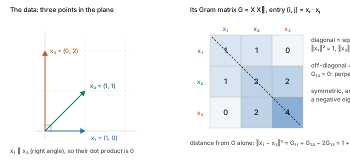
Stack the vectors as the rows of a data matrix X (n rows, one per sample; d columns, one per feature). The running example is three points in the plane:
x_1=(1,0),\quad x_2=(1,1),\quad x_3=(0,2),\qquad X=\begin{bmatrix}1&0\\1&1\\0&2\end{bmatrix}.
Row i of X times column j of X^\top is x_i\cdot x_j, so the whole table is one product:
G = XX^\top=\begin{bmatrix}1&1&0\\1&2&2\\0&2&4\end{bmatrix}.
| Symbol | Read it as | Size |
|---|---|---|
| x_i | the i-th sample (an embedding, a feature vector) | d numbers |
| X | all samples, one per row | n\times d |
| G=XX^\top | Gram matrix: dot products between samples | n\times n |
| X^\top X | dot products between features (an unnormalised covariance) | d\times d |
| K, K_{ij}=k(x_i,x_j) | kernel Gram matrix: a “similarity” in place of the dot product | n\times n |
| H=I-\tfrac1n\mathbf 1\mathbf 1^\top | the centring matrix | n\times n |
A word on convention: some texts stack samples as columns and write G=X^\top X. Nothing changes except the transpose; the question to ask is always “dot products between what?”.
2. What G remembers: lengths, angles, distances
Everything geometric about the set can be read off G:
- Lengths are on the diagonal: \|x_i\|^2=G_{ii}. Here 1,2,4.
- Angles come from normalising: \cos\theta_{ij}=G_{ij}/\sqrt{G_{ii}G_{jj}}. For x_1,x_2 that is 1/\sqrt2\approx0.7071, i.e. 45^\circ; for x_1,x_3 it is 0, a right angle.
- Distances expand like (a-b)^2=a^2+b^2-2ab:
\|x_i-x_j\|^2 = G_{ii}+G_{jj}-2G_{ij}.
So \|x_1-x_3\|^2 = 1+4-0=5, which is indeed \|(1,-2)\|^2.
This last identity is why a Gram matrix and a distance matrix carry the same information (once you fix where the origin is, see §6).
3. What G forgets: which way the cloud faces
Rotate (or reflect) every point by the same orthogonal matrix Q, so X\mapsto XQ. Then
(XQ)(XQ)^\top = X\,QQ^\top X^\top = XX^\top = G.
Rotations do not change lengths or angles, so they cannot change a table of dot products. The code checks this for a 0.7 rad rotation: the largest change in any entry is 4\times10^{-16}, i.e. rounding. The converse also holds and is the useful direction: two point sets with the same Gram matrix differ only by a rotation/reflection. §5 shows how to rebuild them.
For representation learning this is the right invariance. A network’s embedding space has no preferred axes, so any quantity that should not depend on an arbitrary rotation of the features (CKA, kernel methods, InfoNCE logits) is naturally a function of a Gram matrix.
4. Always symmetric, never negative
Two facts hold for every Gram matrix, whatever the data.
Symmetric, because x_i\cdot x_j=x_j\cdot x_i.
Positive semidefinite (PSD): for any weights v=(v_1,\dots,v_n),
v^\top G v = v^\top XX^\top v = \|X^\top v\|^2 = \Big\|\sum_i v_i x_i\Big\|^2 \;\ge\;0.
In words: v^\top Gv is the squared length of the weighted sum \sum_i v_ix_i, and a squared length cannot be negative. Equivalently, every eigenvalue of G is \ge 0. With v=(2,-1,0.5) the sum is 2x_1-x_2+0.5x_3=(1,0), and v^\top Gv=1.
Rank equals the rank of X, so at most \min(n,d). Our three points live in a 2-dimensional plane, so the 3\times3 matrix G has rank 2 and eigenvalues 5.3028,\ 1.6972,\ 0. The zero eigenvalue’s eigenvector is a set of weights with \sum_i v_ix_i=0, a linear dependence among the points. In a batch of n=256 embeddings of dimension d=128, the 256\times256 Gram matrix has at least 128 zero eigenvalues.
The converse is what makes kernels work: any symmetric PSD matrix is the Gram matrix of some set of vectors (§5 builds them). So “is this similarity a legal kernel?” is the same question as “are its Gram matrices always PSD?”.
5. Rebuilding the points from G alone
Diagonalise the symmetric PSD matrix, G=U\Lambda U^\top with \Lambda the (non-negative) eigenvalues. Then set
Y = U\Lambda^{1/2}\quad\Longrightarrow\quad YY^\top=U\Lambda U^\top=G .
The rows of Y are a set of points with exactly the Gram matrix G. Keeping only the top k eigenvalues gives the best k-dimensional approximation (Eckart–Young). For the running example, keeping the two nonzero eigenvalues gives
Y\approx\begin{bmatrix}0.290&-0.957\\1.247&-0.667\\1.914&0.580\end{bmatrix},
which does not look like X but is X rotated: the code finds the 2\times2 map from Y to X and confirms it is orthogonal. This recipe, applied to a double-centred distance matrix, is classical multidimensional scaling (MDS), and applied to a centred G it is exactly PCA scores computed “from the sample side”.
6. Two Gram matrices of one data set: XX^\top and X^\top X
The same X gives two products:
- XX^\top, n\times n: dot products between samples. Here 3\times3.
- X^\top X, d\times d: dot products between features (columns). Here \begin{bmatrix}2&1\\1&5\end{bmatrix}, eigenvalues (7\pm\sqrt{13})/2 = 5.3028,\ 1.6972.
They share their nonzero eigenvalues, and the extra eigenvalues of the bigger one are zero. The reason is the SVD X=U\Sigma V^\top: XX^\top=U\Sigma^2U^\top and X^\top X=V\Sigma^2V^\top, same \Sigma^2. This is the dual view that powers the kernel trick and cheap PCA: when n\ll d (100 images, 2048-dim features), work with the small n\times n Gram matrix instead of the huge d\times d covariance. LogME uses exactly this switch when features outnumber samples.
Centring. Covariance needs the mean removed. On the sample side that is the centring matrix H=I-\tfrac1n\mathbf 1\mathbf 1^\top:
HGH = (HX)(HX)^\top = \text{Gram matrix of the mean-subtracted points}.
Its rows sum to zero, so \mathbf 1 is always in its null space. HGH is the object in HSIC, CKA and kernel PCA.
7. Kernels: a Gram matrix with a different “dot product”
Replace x_i\cdot x_j with a similarity k(x_i,x_j). If k is a kernel, meaning k(x,y)=\phi(x)\cdot\phi(y) for some feature map \phi (possibly infinite-dimensional), then K_{ij}=k(x_i,x_j) is still a Gram matrix, of the vectors \phi(x_i), and §§2–6 all apply. You never need to compute \phi: that is the kernel trick.
The workhorse is the RBF (Gaussian) kernel k(x,y)=\exp(-\|x-y\|^2/2\sigma^2). Its bandwidth \sigma decides how far “similar” reaches:
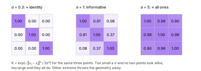
At either extreme the matrix stops depending on the data: near-identity means every point looks unrelated, near-all-ones means every point looks the same. This is why kernel scores (MMD, HSIC) are sensitive to \sigma and why the “median distance” heuristic exists.
The NTK is a Gram matrix of gradients. For a network f(x;\theta), set \phi(x)=\nabla_\theta f(x;\theta), one long vector per input. Then
\Theta_{ij}=\nabla_\theta f(x_i)\cdot\nabla_\theta f(x_j)
is the empirical NTK: the Gram matrix of per-example gradients. It is PSD for the reason in §4, and its eigenvectors are the directions in function space that gradient descent learns fast (large eigenvalue) or slowly (small).
8. Where it shows up in the paper notes
| Where | Which Gram matrix | What it is used for |
|---|---|---|
| NTK (Jacot et al.), deep vs. kernel (Fort et al.) | gradients, \Theta=JJ^\top | training dynamics are linear in \Theta; its spectrum sets learning speed per direction |
| NTK-Selector (Wang et al.) | gradient Gram between general and domain data | picks general examples whose gradients align with the small domain set |
| InfoNCE (Betser et al.), alignment/uniformity | normalised embeddings, ZZ^\top/\tau | row-wise softmax of the cosine Gram matrix is the contrastive loss; uniformity is an RBF-kernel mean over it |
| Spectral contrastive (HaoChen et al.) | augmentation-graph adjacency | the loss is a low-rank factorisation \approx FF^\top of a normalised graph matrix |
| H-score, LogME | X^\top X (feature side) and XX^\top (sample side) | covariance of features; LogME’s dual switch when d>n |
| Four subspaces | A^\top A | normal equations, and why it squares the condition number (§9) |
A further standard use not covered by a paper here: neural style transfer compares the C\times C Gram matrix of a CNN layer’s channels (dot products between channel activation maps, summed over pixels). Summing over positions throws away where things are and keeps which features co-occur, which is what “style” turns out to be.
9. A numerical caution
Forming X^\top X (or XX^\top) squares the condition number: its eigenvalues are the squared singular values of X. In the code, a 50\times5 matrix with one column shrunk by 10^{-3} has \mathrm{cond}(A)\approx967 and \mathrm{cond}(A^\top A)\approx9.35\times10^{5}. In float32 (about 7 significant digits) that is most of the precision gone. Hence: solve least squares with QR or SVD rather than the normal equations, and add a small ridge \lambda I to a kernel Gram matrix before inverting it.
Questions and doubts
- The PSD guarantee is exact in maths but not in floating point: a large kernel matrix routinely reports tiny negative eigenvalues. Clipping them, or adding jitter, is standard, but how much jitter changes an MMD or CKA value is rarely reported.
- CKA compares two networks via their centred Gram matrices and is invariant to rotations and isotropic scaling of features. Is that invariance always wanted? Two layers that differ by an anisotropic rescaling look different to CKA, though a linear probe would not care.
- The empirical NTK Gram matrix is n\times n but each entry needs two gradients of full parameter size. The low-rank or random-projection approximations used in practice (and in NTK-Selector) change which eigen-directions survive; worth checking against the exact one on a small model.
Takeaways
- A Gram matrix is a table of dot products, G=XX^\top. Diagonal: squared lengths. Off-diagonal: dot products. Distances: G_{ii}+G_{jj}-2G_{ij}.
- It keeps all the shape of the point set and forgets only its orientation; the points can be rebuilt from it up to a rotation.
- It is always symmetric PSD, rank \le\min(n,d), and shares its nonzero eigenvalues with X^\top X. Pick whichever side is smaller.
- Kernel matrices, the NTK and contrastive similarity matrices are all Gram matrices of some feature map, so the same facts apply to each of them.