Variational Bayes: the KL split, mean-field updates, and a worked Normal example
Links
- Paper being read: Tran, Nguyen and Dao, A practical tutorial on Variational Bayes, 2021. arXiv abstract · PDF. These notes follow its opening pages and its Example 2.1, and fill in the steps it skips.
- The ELBO: the same bound derived from Jensen’s inequality, with the two-coin example. Here the bound is reached by splitting the KL instead.
- Expectation–Maximization: the E-step chooses q exactly, which is the special case of VB where the posterior is tractable.
- The reparameterization trick: how the gradients used by fixed-form VB (§4) are estimated.
code/mfvb_normal.pyprints every number quoted in §8 and, with--figures, redraws the three figures.
In one paragraph
Bayesian inference wants the posterior p(\theta\mid y)=p(\theta)p(y\mid\theta)/p(y), but the normaliser p(y)=\int p(\theta)p(y\mid\theta)\,d\theta is usually an integral we cannot do. Variational Bayes (VB) replaces the posterior by the closest member q^* of a family \mathcal Q of tractable distributions, where “closest” means smallest \mathrm{KL}(q\|p(\cdot\mid y)). The KL itself contains the intractable p(y), but it only enters as an additive constant, so minimising the KL over q is exactly the same as maximising a quantity, the ELBO, that never needs p(y). All of the approximation error comes from restricting q to \mathcal Q.
1. Questions, in plain words and in symbols
| # | Plain-language question | Mathematical question |
|---|---|---|
| 1 | The distance between my guess and the true posterior mentions the very number I cannot compute. How can I minimise it? | Show \mathrm{KL}(q\|p(\cdot\mid y))=-\int q\log\frac{p(\theta)p(y\mid\theta)}{q}\,d\theta+\log p(y). |
| 2 | Is swapping the distance for the computable part an approximation? | Is \arg\min_q\mathrm{KL}=\arg\max_q\mathrm{ELBO} exact? Where does the approximation enter? |
| 3 | What does “assume the pieces are independent” cost, and what are the alternatives? | Define the mean-field family; compare it with fixed-form VB and normalizing flows. |
| 4 | With two independent pieces, how do I improve one while the other is frozen? | Write the ELBO for q_1q_2, isolate q_1, and find \arg\max_{q_1}. |
| 5 | When does each update land in a familiar distribution? | State conditional conjugacy and show q_1 stays in the prior’s family. |
| 6 | Does all of this really work on a small problem? | Run it on Example 2.1 and compare with the exact posterior. |
Notation
| Symbol | Meaning |
|---|---|
| y | observed data |
| \theta | unknown parameters (\theta=(\theta_1,\dots,\theta_d) when split into blocks) |
| p(\theta), p(y\mid\theta) | prior, likelihood |
| p(\theta\mid y) | posterior =p(\theta)p(y\mid\theta)/p(y) |
| p(y) | evidence =\int p(\theta)p(y\mid\theta)\,d\theta, the intractable normaliser |
| q(\theta) | the approximating density; \mathcal Q is the family it is chosen from |
| \mathrm{ELBO}(q) | \int q(\theta)\log\frac{p(\theta)p(y\mid\theta)}{q(\theta)}\,d\theta (the paper writes \mathrm{LB}) |
| E_{-\theta_1}[\cdot] | average over every block except \theta_1, under the current q of those blocks |
2. Question 1: the KL splits into two pieces
Start from the definition and substitute Bayes’ rule inside the logarithm.
\mathrm{KL}(q\,\|\,p(\cdot\mid y))=\int q(\theta)\log\frac{q(\theta)}{p(\theta\mid y)}\,d\theta,\qquad p(\theta\mid y)=\frac{p(\theta)p(y\mid\theta)}{p(y)}.
Plugging in, the ratio becomes \log\frac{q(\theta)}{p(\theta\mid y)}=\log\frac{q(\theta)\,p(y)}{p(\theta)p(y\mid\theta)} =\log\frac{q(\theta)}{p(\theta)p(y\mid\theta)}+\log p(y), using \log(ab)=\log a+\log b. Integrate against q, term by term:
- the first term is \int q\log\frac{q}{p(\theta)p(y\mid\theta)}\,d\theta=-\int q\log\frac{p(\theta)p(y\mid\theta)}{q}\,d\theta, because swapping numerator and denominator flips the sign of a logarithm;
- the second term does not involve \theta, so it leaves the integral, and \int q\,d\theta=1 leaves exactly \log p(y).
\boxed{\ \mathrm{KL}(q\|p(\cdot\mid y))=-\mathrm{ELBO}(q)+\log p(y)\ } \qquad\Longleftrightarrow\qquad \log p(y)=\mathrm{ELBO}(q)+\mathrm{KL}(q\|p(\cdot\mid y)).
The ELBO involves only the prior, the likelihood and q, all of which we can evaluate. \log p(y) is the part we cannot compute, and it does not depend on q.
3. Question 2: exact, not an approximation
Because \log p(y) is a constant in q, every increase of the ELBO is an equal decrease of the KL. So for any family \mathcal Q, \arg\min_{q\in\mathcal Q}\mathrm{KL}(q\|p(\cdot\mid y))=\arg\max_{q\in\mathcal Q}\mathrm{ELBO}(q). Since \mathrm{KL}\ge0, also \mathrm{ELBO}(q)\le\log p(y), which is where the name (evidence lower bound) comes from.
The approximation is the restriction q\in\mathcal Q.
- If the true posterior lies in \mathcal Q, the minimum KL is 0 and q^* is the posterior; the ELBO equals \log p(y).
- Otherwise the minimum KL is positive, q^* is the closest member of \mathcal Q, and \log p(y)-\mathrm{ELBO}(q^*) is that leftover KL.
One more thing is fixed by the objective, not by \mathcal Q: the KL is taken in the order \mathrm{KL}(q\|p), the “reverse” direction, which tends to make q^* settle on one region of the posterior and understate its spread. §8 shows this on a real example (the standard deviation of \mu).
4. Question 3: choosing the family \mathcal Q
Mean-field. \mathcal Q is every q that factorises across blocks of parameters: q(\theta)=q_1(\theta_1)\,q_2(\theta_2)\cdots q_d(\theta_d). The form of each factor is not chosen; it falls out of the optimisation (§6). The price is that the dependence between blocks in the true posterior is thrown away. If the true posterior of two parameters is a tilted ellipse, the best product is an axis-aligned blob, so it cannot tilt.
Fixed-form VB (FFVB) and mean-field VB (MFVB) are the two classes the paper distinguishes. They differ in how \mathcal Q is specified and fitted, not in the objective:
| MFVB | FFVB | |
|---|---|---|
| What is restricted | q factorises | q has a parametric form chosen in advance (e.g. a Gaussian N(\mu,\Sigma)) |
| Form of each factor | determined by the model | chosen by you |
| Dependence between coordinates | none | possible (a full-covariance Gaussian keeps it) |
| Optimisation | coordinate ascent, closed-form updates | stochastic gradient ascent on the parameters of q |
| Needs | model-specific derivation | only the ability to evaluate \log p(\theta)p(y\mid\theta) |
They can overlap: a diagonal Gaussian fitted by gradients is fixed-form and mean-field in structure.
Normalizing flows are a very flexible fixed form. Take a simple base density q_0(z) and an invertible, differentiable map T_\phi, set \theta=T_\phi(z), and the density is exact: q_\phi(\theta)=q_0(z)\,\bigl|\det\partial T_\phi/\partial z\bigr|^{-1},\quad z=T_\phi^{-1}(\theta). If T_\phi mixes coordinates, q_\phi has dependence between them; if it acts coordinate by coordinate, you get a mean-field q. So mean-field is one end of the scale (cheap, restrictive) and a rich flow is the other (expensive, nearly unrestricted).
5. Question 4: the ELBO for two factors
Take \theta=(\theta_1,\theta_2) and q=q_1q_2. Write \log p(\theta,y) for \log p(\theta)p(y\mid\theta).
\mathrm{ELBO}(q_1,q_2)=\iint q_1q_2\log p(\theta,y)\,d\theta_1d\theta_2-\iint q_1q_2\log(q_1q_2)\,d\theta_1d\theta_2.
The entropy term splits. \log(q_1q_2)=\log q_1+\log q_2. In \iint q_1q_2\log q_1 the factor q_1\log q_1 does not involve \theta_2, so it leaves the inner integral, which is \int q_2\,d\theta_2=1: \iint q_1q_2\log(q_1q_2)=\int q_1\log q_1\,d\theta_1+\int q_2\log q_2\,d\theta_2. (The entropy of independent pieces is the sum of their entropies.)
The first term, as an iterated integral. \iint q_1q_2\log p(\theta,y)=\int q_1(\theta_1)\Bigl[\int q_2(\theta_2)\log p(\theta,y)\,d\theta_2\Bigr]d\theta_1 =\int q_1(\theta_1)\,E_{-\theta_1}[\log p(y,\theta)]\,d\theta_1, where E_{-\theta_1}[\log p(y,\theta)]:=E_{q_2}[\log p(y,\theta)] is a function of \theta_1 only, since \theta_2 has been averaged out.
Putting the pieces together, \mathrm{ELBO}(q_1,q_2)=\int q_1E_{-\theta_1}[\log p(y,\theta)]\,d\theta_1-\int q_1\log q_1\,d\theta_1+C(q_2), \qquad C(q_2)=-\int q_2\log q_2\,d\theta_2.
C(q_2) is “a constant” only with respect to q_1: the ELBO still depends on both factors. In coordinate ascent q_2 is frozen while q_1 is updated, then the roles swap, and the term that was a constant becomes the one being optimised.
Merging the q_1 terms (linearity of the integral, \int f-\int g=\int(f-g)), then using x=\log e^x and \log a-\log b=\log(a/b): \mathrm{ELBO}=\int q_1\Bigl\{E_{-\theta_1}[\log p(y,\theta)]-\log q_1\Bigr\}d\theta_1+C(q_2) =\int q_1\log\frac{\exp\bigl(E_{-\theta_1}[\log p(y,\theta)]\bigr)}{q_1}\,d\theta_1+C(q_2).
This has the shape of the ELBO from §2. The function in the numerator is not a density yet; normalise it, q_1^*(\theta_1)=\frac{\exp(E_{-\theta_1}[\log p(y,\theta)])}{Z},\qquad Z=\int\exp(E_{-\theta_1}[\log p(y,\theta)])\,d\theta_1, and the q_1-part of the ELBO equals -\mathrm{KL}(q_1\|q_1^*)+\log Z. The KL is smallest (zero) at q_1=q_1^*, so \boxed{\ \log q_1^*(\theta_1)=E_{-\theta_1}[\log p(y,\theta)]+\text{const}\ } is the exact best q_1 given q_2, and the same holds for every block.
Why coordinate ascent here, rather than gradient ascent.
- each update is the exact maximiser over one block, so there is no step size to tune and the ELBO never goes down;
- the unknown is a whole function q_1, and the formula gives it directly, with no parametric form to choose first;
- for conditionally conjugate models the update is an explicit formula (§7).
Gradient ascent is used when this expectation has no closed form, when q must keep dependence between coordinates, or when minibatches are needed for large data: that is FFVB. The weakness of coordinate ascent is that it zigzags when coordinates are strongly dependent in the true posterior.
6. Question 5: conjugacy, and why q_1 stays in the prior’s family
A prior is conjugate to a likelihood if their product is in the prior’s family. Beta prior, Bernoulli likelihood: \theta^{a-1}(1-\theta)^{b-1}\cdot\theta^h(1-\theta)^{n-h}\propto\theta^{a+h-1}(1-\theta)^{b+n-h-1} is Beta(a+h,\,b+n-h) again, with updated numbers. A model is conditionally conjugate if each block, given all the others, has this property.
In the update \log q_1^*=E_{-\theta_1}[\log p(y,\theta)]+\text{const}, only the terms with \theta_1 matter, so \log q_1^*=E_{q_2}[\log p(\theta_1\mid\theta_2,y)]+\text{const}. If the full conditional is an exponential-family member of the prior’s family, \log p(\theta_1\mid\theta_2,y)=\eta(\theta_2,y)^\top T(\theta_1)+\log h(\theta_1)+\text{const}, then only \eta involves \theta_2, and the average over q_2 just replaces \eta by E_{q_2}[\eta]: q_1^*(\theta_1)\propto h(\theta_1)\exp\bigl(E_{q_2}[\eta]^\top T(\theta_1)\bigr), the same family with the “expected parameters”. Without conditional conjugacy, \log p(\theta_1\mid\theta_2,y) is not of this form, q_1^* is not a recognisable distribution, and the exact update is not available.
7. Example 2.1 set up
Ten observations y=(11,12,8,10,9,8,9,10,13,7) from N(\mu,\sigma^2), with priors \mu\sim N(\mu_0,\sigma_0^2), \sigma^2\sim\text{Inverse-Gamma}(\alpha_0,\beta_0), and \mu_0=0, \sigma_0^2=100, \alpha_0=\beta_0=1. Factorise q(\mu,\sigma^2)=q(\mu)q(\sigma^2). The model is conditionally conjugate (a Normal given \sigma^2, an Inverse-Gamma given \mu) but not jointly conjugate, so the posterior has no closed form, which is why VB is used.
Update for q(\mu)=N(m,s^2). Keep the \mu-terms of \log p(y,\mu,\sigma^2) and average \sigma^2 out; it appears only through \tau:=E_{q(\sigma^2)}[1/\sigma^2]. \log q(\mu)=-\tfrac{\tau}{2}\sum_i(y_i-\mu)^2-\frac{(\mu-\mu_0)^2}{2\sigma_0^2}+\text{const} =-\tfrac12\mu^2\Bigl(n\tau+\tfrac1{\sigma_0^2}\Bigr)+\mu\Bigl(\tau\textstyle\sum y_i+\tfrac{\mu_0}{\sigma_0^2}\Bigr)+\text{const}. A N(m,s^2) has log-density -\mu^2/(2s^2)+\mu m/s^2+\text{const}. Matching coefficients: \frac1{s^2}=n\tau+\frac1{\sigma_0^2},\qquad m=s^2\Bigl(\tau\sum y_i+\frac{\mu_0}{\sigma_0^2}\Bigr). The data precision n\tau adds to the prior precision, and m is a precision-weighted average of data and prior mean.
Update for q(\sigma^2)=\text{IG}(\alpha,\beta). Keep the \sigma^2-terms and average \mu out: \log q(\sigma^2)=-\Bigl(\alpha_0+\tfrac n2+1\Bigr)\log\sigma^2-\frac{\beta_0+\tfrac12E_{q(\mu)}\sum_i(y_i-\mu)^2}{\sigma^2}+\text{const}. Under q(\mu)=N(m,s^2), E[(y_i-\mu)^2]=(y_i-m)^2+s^2, so E\sum(y_i-\mu)^2=\sum(y_i-m)^2+ns^2. The extra ns^2 is the price of not knowing \mu exactly. Matching -(\alpha+1)\log\sigma^2-\beta/\sigma^2: \alpha=\alpha_0+\tfrac n2,\qquad \beta=\beta_0+\tfrac12\Bigl[\sum_i(y_i-m)^2+ns^2\Bigr],\qquad \tau=E[1/\sigma^2]=\alpha/\beta. The two factors pass information through \tau (from q(\sigma^2) to q(\mu)) and through (m,s^2) (the other way). \alpha=6 never changes; \beta moves until m and s^2 settle.
8. The code, line by line
code/mfvb_normal.py implements §7 and checks it against
the exact posterior on a grid. The comments in the file carry the same
explanations as below.
| Code | What it does |
|---|---|
s2 = 1/(n*tau + 1/s0sq) |
s^2: data precision n\tau plus prior precision 1/\sigma_0^2, inverted |
m = s2*tau*y.sum() |
m=s^2(\tau\sum
y_i+\mu_0/\sigma_0^2) with the \mu_0 term dropped because \mu_0=0 (a nonzero \mu_0 needs + mu0/s0sq inside
the bracket) |
a = a0 + n/2 |
\alpha=\alpha_0+n/2=6, fixed |
b = b0 + 0.5*(((y-m)**2).sum() + n*s2) |
\beta: the residual sum of squares around m plus ns^2 for the uncertainty in \mu |
tau = a/b |
E[1/\sigma^2] under \text{IG}(\alpha,\beta), fed into the next sweep |
M, S = np.meshgrid(mu, sg) |
two arrays holding \mu and \sigma^2 at every grid point, so each density is evaluated at all points at once |
lp = norm_logpdf(M, mu0, s0sq) + ig_logpdf(S, a0, b0) |
log prior of \mu plus log prior of \sigma^2 |
lp = lp + norm_logpdf(yi, M, S) per data point |
adds the log-likelihood (a sum, since observations are independent);
lp is then \log
p(\mu,\sigma^2,y), the true log-posterior up to the constant
\log p(y) |
P = np.exp(lp - lp.max()) |
exponentiate; subtracting the maximum first avoids underflow and only rescales by a constant |
P / (P.sum() * dmu * dsg) |
normalise by a Riemann sum of \iint P, a numerical stand-in for the intractable p(y); the result integrates to about 1 |
mean_field_density(...) |
q(\mu)q(\sigma^2) on the same grid; already normalised, since each factor is |
P.sum(0)*dsg, P.sum(1)*dmu |
exact marginals of \mu and \sigma^2: sum the grid over the other variable |
9. Results
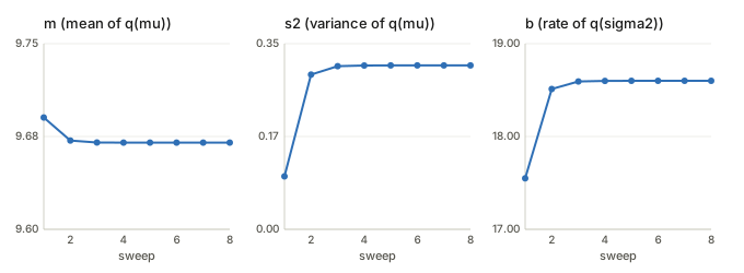
Running the script gives, for the first sweeps and at convergence:
| sweep | m | s^2 | \alpha | \beta |
|---|---|---|---|---|
| 1 | 9.6903 | 0.0999 | 6 | 17.5500 |
| 2 | 9.6717 | 0.2916 | 6 | 18.5122 |
| 3 | 9.6702 | 0.3076 | 6 | 18.5924 |
| 5 | 9.6700 | 0.3090 | 6 | 18.5996 |
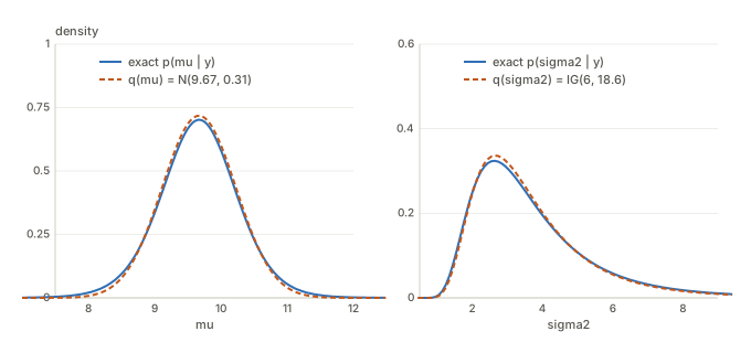
So q(\mu)=N(9.670,\,0.309) and q(\sigma^2)=\text{IG}(6,\,18.60), after about five sweeps.
Against the exact posterior on a grid:
| exact | VB | |
|---|---|---|
| E[\mu] | 9.664 | 9.670 |
| sd of \mu | 0.611 | 0.556 |
| E[\sigma^2] | 3.784 | 3.720 |
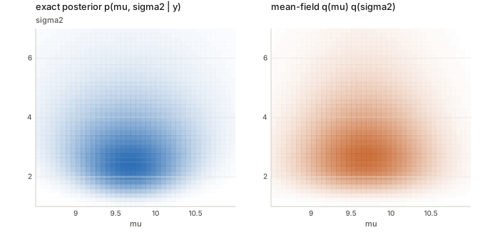
- The exact posterior correlation of (\mu,\sigma^2) is -0.028, essentially zero. That is why a product loses little here: the contours are nearly axis-aligned already.
- The marginals nearly coincide. The visible difference is in the spread: VB’s \mu has standard deviation 0.556 against the exact 0.611, about 9% too narrow, the under-dispersion that the reverse KL tends to produce (§3).
Questions and doubts
- How general is the under-dispersion? Here the loss is small because the posterior is nearly uncorrelated. I have only checked this one example; with strongly correlated parameters I would expect mean-field to understate marginal spread by much more, but I have not tested it.
- Local optima. Each coordinate update is exact, and the ELBO never decreases, but the ELBO need not be concave in (q_1,q_2) jointly. For this model I started the loop from \tau=0.001, 1 and 100 and all reach the same fixed point (m=9.670, s^2=0.309, \beta=18.60 after 100 sweeps), but that says nothing about models with several local optima.
- The \mu_0 term.
The script’s
mline drops \mu_0/\sigma_0^2 because \mu_0=0. The general formula is in the table of §8 but I have not run a case with \mu_0\neq0. - Grid truncation. The \sigma^2 grid ends at 60, since the Inverse-Gamma tail is heavy; with a grid ending at 9 the exact E[\sigma^2] came out as 3.59 instead of 3.78, so the exact column above depends on the grid reaching far enough.
- Only the opening pages and Example 2.1 were read. I have not worked through the paper’s later sections (the general MFVB procedure and the FFVB algorithms), so the FFVB row in §4 reflects the usual meaning of “fixed-form VB”, which I matched against the paper’s one defining sentence only.
- What would a tighter family buy? A full-covariance Gaussian or a flow would recover the correlation, but on this example the correlation is already about zero, so the extra cost would buy almost nothing; whether that holds with more parameters is not examined.
Cheat sheet
- Posterior: p(\theta\mid y)=p(\theta)p(y\mid\theta)/p(y), with p(y) intractable.
- Exact identity: \log p(y)=\mathrm{ELBO}(q)+\mathrm{KL}(q\|p(\cdot\mid y)), with \mathrm{ELBO}(q)=\int q\log\frac{p(\theta)p(y\mid\theta)}{q}\,d\theta.
- Maximising the ELBO over q\in\mathcal Q is exactly minimising the KL; the approximation is q\in\mathcal Q.
- Mean-field: q=\prod_jq_j(\theta_j); entropy of the product is the sum of the entropies.
- Optimal factor: \log q_j^*(\theta_j)=E_{-\theta_j}[\log p(y,\theta)]+\text{const}; coordinate ascent cycles through the j.
- Conditional conjugacy: q_j^* is in the prior’s family with parameters replaced by their expectations under the other factors.
- Example 2.1: 1/s^2=n\tau+1/\sigma_0^2, m=s^2(\tau\sum y+\mu_0/\sigma_0^2), \alpha=\alpha_0+n/2, \beta=\beta_0+\frac12[\sum(y-m)^2+ns^2], \tau=\alpha/\beta; converges to N(9.670,0.309) and \text{IG}(6,18.60).