Inequalities and Concentration: a working toolbox
Background for the annotations in this repo. Every paper here is ultimately a chain of inequalities, and the same dozen tools recur. This page collects them with statements, the intuition, where each one is used, and — where it is cheap to do so — a numerical check.
It is organised by what a tool is for, not by field, because that is how you reach for one:
- Concentration — a random quantity is close to its mean. How close, how often?
- Comparison — bound one quantity you cannot compute by another you can.
- Geometry ↔︎ spectrum — relate a combinatorial quantity (cuts, partitions) to an algebraic one (eigenvalues). Cheeger’s inequality and its relatives.
- Perturbation — the input moved a little; how far did the answer move?
- Limits — the exact distribution is intractable; what does it converge to, and how fast?
Where each tool gets used
A cross-reference for the papers annotated here. Details for each row are in the sections below.
| Tool | Used in | For what |
|---|---|---|
| Cauchy–Schwarz | Betser Prop. 1 (twice) | bounding \mathbb{E}[gh], then summing over coordinates |
| HGR maximal correlation + DPI | Betser Prop. 1 | the alignment ceiling \eta_2 |
| Donsker–Varadhan | Betser Lem. 1; Zhang Lem. B.2 | lower-bounding \mathrm{KL}(\mu\Vert\sigma) by \lVert m(\mu)\rVert^2 |
| KL chain rule | Betser Prop. 3; Zhang Prop. 3 | splitting radial from angular |
| Concentration on the sphere | Betser Lem. 1, Asm. 2 | the constant in Lemma 1; thin-shell |
| Maxwell–Poincaré CLT | Betser Cor. 1 | uniform on S^{d-1} \Rightarrow Gaussian projections |
| Diaconis–Freedman rate | Betser Thm. 2 | d_{\mathrm{TV}} \le 2(k+3)/(d-k-3) |
| Slutsky | Betser Prop. 2 | lifting the sphere result to \mathbb{R}^d |
| Berry–Esseen | Betser, discussion | finite-d rates |
| Cheeger’s inequality | HaoChen (via \rho_m); Zhang (inherited) | conductance \leftrightarrow spectral gap |
| Higher-order Cheeger | HaoChen Thm. 3.7 | \rho_m \leftrightarrow \lambda_m, hence the \rho^2 |
| Eckart–Young–Mirsky | HaoChen Lem. 3.1–3.2 | minimiser of \lVert\bar A - FF^\top\rVert_F^2 is the top eigenvectors |
| Rademacher + symmetrisation | HaoChen Thm. 4.1 | finite-sample bound on the population loss |
| Bounded differences | HaoChen Thm. 4.1, 5.1 | the \sqrt{\log(1/\delta)/n} terms |
| Davis–Kahan (in spirit) | HaoChen Thm. 4.2 | why the bound has k\epsilon/\Delta |
| Weyl’s inequality | Zhang §B.3 | effect of the \epsilon W perturbation |
| Wigner semicircle law | Zhang §B.3, Thm. B.4 | spectrum of the noise; the Kepler-equation term |
| Jensen | everywhere, implicitly | convexity of \log\sum\exp; \Phi(\mu) \ge \Phi(\sigma) |
1. Comparison: the workhorses
Cauchy–Schwarz
\lvert \langle a, b\rangle \rvert \le \lVert a\rVert \cdot \lVert b \rVert, \qquad\text{or}\qquad \big(\mathbb{E}[XY]\big)^2 \le \mathbb{E}[X^2]\,\mathbb{E}[Y^2].
Equality iff a and b are parallel. Unremarkable until you notice how much work it does. In Betser et al.’s Proposition 1 it appears twice, in different guises, and seeing the difference is instructive:
- As an expectation bound. \mathbb{E}[g(X)h(Y)] \le \rho_m \sqrt{\operatorname{Var}(g)\operatorname{Var}(h)} — Cauchy–Schwarz in L^2(\mathbb{P}), with the HGR constant improving the naive bound.
- As a sequence bound. \sum_k \sqrt{a_k b_k} \le \sqrt{\sum_k a_k}\sqrt{\sum_k b_k} — the same inequality in \ell^2, applied to the vector of per-coordinate variances.
A useful habit: whenever a proof sums a product over an index, expect Cauchy–Schwarz to collapse it into a product of two norms.
Jensen’s inequality
For convex \varphi: \varphi(\mathbb{E}[X]) \le \mathbb{E}[\varphi(X)], reversed for concave \varphi.
This is the silent partner in every contrastive-learning proof, because \log\sum\exp is convex. It is why Betser et al.’s uniformity potential \Phi(\mu) = \mathbb{E}_u \log \mathbb{E}_v \exp(\alpha u\cdot v) has a minimum at the uniform law rather than a maximum, and why swapping an expectation past a \log is a move that costs you something in a known direction.
Markov → Chebyshev → Chernoff: the concentration ladder
Each rung buys sharper tails by assuming more.
| Assume | Bound | Tail |
|---|---|---|
| X \ge 0 | \Pr[X \ge t] \le \mathbb{E}[X]/t (Markov) | 1/t |
| finite variance | \Pr[\lvert X - \mu\rvert \ge t] \le \sigma^2/t^2 (Chebyshev) | 1/t^2 |
| bounded / sub-gaussian MGF | \Pr[\lvert \bar X - \mu \rvert \ge t] \le 2e^{-2nt^2/(b-a)^2} (Hoeffding) | e^{-nt^2} |
The jump from polynomial to exponential is what makes learning theory work at all: it is the difference between needing O(1/\epsilon^2\delta) samples and O(\log(1/\delta)/\epsilon^2). Chebyshev follows from Markov applied to (X-\mu)^2; Chernoff-type bounds follow from Markov applied to e^{\lambda X} and then optimising \lambda. Every concentration bound in these papers is Markov’s inequality applied to a cleverly chosen function.
McDiarmid / bounded differences
If f(x_1,\dots,x_n) changes by at most c_i when coordinate i alone changes, then
\Pr\big[\lvert f - \mathbb{E}f\rvert \ge t\big] \le 2\exp\!\left(\frac{-2t^2}{\sum_i c_i^2}\right).
The generalisation of Hoeffding from sums to any stable function, which is what you need for a supremum over a hypothesis class. This is the source of the \sqrt{\log(2/\delta)/n} term in HaoChen et al.’s Theorem 4.1 and the \sqrt{\log(1/\delta)/n} in Theorem 5.1. When you see that shape, McDiarmid or Hoeffding is underneath.
Rademacher complexity and symmetrisation
\hat{\mathcal{R}}_n(\mathcal{F}) := \mathbb{E}_\varepsilon\left[\sup_{f\in\mathcal{F}} \frac{1}{n}\sum_{j=1}^n \varepsilon_j f(x_j)\right], \qquad \varepsilon_j \in \{\pm 1\} \text{ uniform},
measuring how well the class can correlate with pure noise — its effective capacity. The symmetrisation lemma says the generalisation gap is controlled by it:
\mathbb{E}\left[\sup_{f} \big(\mathbb{E}f - \hat{\mathbb{E}}_n f\big)\right] \le 2\,\hat{\mathcal{R}}_n(\mathcal{F}).
Combine with McDiarmid for the high-probability version, and you have the standard two-term bound: empirical risk + capacity + confidence. HaoChen et al. extend it to vector-valued f by taking the worst output coordinate, which is why their constants carry factors of k.
An important precondition, easy to skip past: symmetrisation needs an unbiased empirical estimator. This is exactly why HaoChen et al. can close the finite-sample gap for the spectral contrastive loss but not for InfoNCE — the spectral loss’s empirical version is unbiased (their negative term averages over the n(n-1) ordered pairs i \ne j for precisely this reason), whereas InfoNCE’s batch denominator is biased at finite batch size. The choice of loss is not cosmetic; it is what makes the standard toolbox applicable.
2. Information-theoretic tools
KL divergence, and the chain rule
\mathrm{KL}(P\Vert Q) = \int \log\frac{dP}{dQ}\,dP \ge 0, zero iff P = Q. Not a metric — asymmetric, no triangle inequality — but it decomposes beautifully, which is what matters here. The chain rule under a disintegration P(dz) = P_1(dx)\,P_2(dy\mid x):
\mathrm{KL}(P\Vert Q) = \mathrm{KL}(P_1\Vert Q_1) + \int \mathrm{KL}\big(P_2(\cdot\mid x)\,\Vert\, Q_2(\cdot\mid x)\big)\,P_1(dx).
Both Betser et al. and Zhang et al. use exactly this to split a law on \mathbb{R}^d into angular and radial parts. The payoff is always the same: the second term is \ge 0 and can be zeroed by matching the conditional, which removes a whole dimension of the optimisation for free. Whenever an objective sees only part of a decomposition, look for a chain rule to solve the invisible part in closed form.
Donsker–Varadhan variational formula
\mathrm{KL}(\mu\Vert\sigma) = \sup_{\varphi}\Big\{\mathbb{E}_{u\sim\mu}[\varphi(u)] - \log\mathbb{E}_{u\sim\sigma}\big[e^{\varphi(u)}\big]\Big\}.
KL as a supremum over test functions. This is the single most useful identity for getting lower bounds on KL, because a supremum is bounded below by any particular choice — pick a convenient \varphi and you are done, with no need to evaluate the divergence.
Both Betser et al. (Lemma 1) and Zhang et al. (Lemma B.2) use it the same way: choose \varphi linear in the direction of the mean, \varphi(u) = t\,\langle m(\mu)/\lVert m(\mu)\rVert, u\rangle, so the first term is t\lVert m(\mu)\rVert and the second is the log-MGF of a spherical marginal — which sub-gaussian concentration on the sphere bounds by O(t^2/d). Optimising t yields
\mathrm{KL}(\mu\Vert\sigma) \ge C(d-1)\lVert m(\mu)\rVert^2 .
The (d-1) is the whole point of Betser et al.’s Theorem 1: it grows with dimension, so the KL penalty for being off-centre outgrows the \alpha(1-\eta_2)\lVert m\rVert^2 alignment reward, and the uniform law wins in high dimensions.
Pinsker’s inequality
d_{\mathrm{TV}}(P,Q) \le \sqrt{\tfrac{1}{2}\mathrm{KL}(P\Vert Q)}.
The standard bridge from KL to total variation, i.e. from an information quantity to a probability of distinguishing. Not invoked explicitly in these three papers, but it is the reason KL bounds are worth having at all — and note the square root, the same loss of sharpness that appears in Cheeger.
HGR maximal correlation and its data-processing inequality
\rho_m(X,Y) = \sup_{\substack{\mathbb{E}\varphi = \mathbb{E}\psi = 0\\ \operatorname{Var}\varphi = \operatorname{Var}\psi = 1}} \mathbb{E}[\varphi(X)\psi(Y)] \in [0,1].
Pearson correlation after optimal nonlinear reshaping of both variables. Unlike Pearson, \rho_m = 0 iff X \perp Y. Its defining property gives, for any mean-zero square-integrable g, h,
\mathbb{E}[g(X)h(Y)] \le \rho_m(X,Y)\sqrt{\operatorname{Var}(g)\operatorname{Var}(h)},
a strict improvement on plain Cauchy–Schwarz whenever \rho_m < 1.
The multiplicative data-processing inequality is what makes it powerful: for a Markov chain X - Y - Z,
\rho_m(X,Z) \le \rho_m(X,Y)\,\rho_m(Y,Z).
Dependence decays multiplicatively along a chain. Betser et al. apply it to X \leftarrow X_0 \rightarrow Y (two views of one base image) to get \rho_m(X,Y) \le \sqrt{\eta_2}\cdot\sqrt{\eta_2} = \eta_2 — a hard ceiling on positive-pair alignment that no encoder can beat. Worth contrasting with mutual information, which also obeys a DPI but an additive one; the multiplicative form is what produces a clean multiplicative ceiling here.
3. Geometry ↔︎ spectrum: Cheeger and relatives
This is the family that lets you convert statements about cuts into statements about eigenvalues, and it is the backbone of the augmentation-graph papers.
Conductance
For a vertex set S, with \operatorname{vol}(S) = \sum_{x\in S} w_x:
\phi(S) = \frac{\text{weight leaving } S}{\operatorname{vol}(S)}, \qquad h(G) = \min_{S} \frac{\text{cut}(S)}{\min\{\operatorname{vol}(S), \operatorname{vol}(S^c)\}}.
h(G) is the Cheeger constant: the best bottleneck in the graph. Small h means a good sparse cut exists. Computing it exactly is NP-hard in general — which is the entire motivation for what follows.
A practical note from checking this numerically: the equivalent definition “minimise \phi(S) over S with \operatorname{vol}(S) \le \operatorname{vol}(V)/2” has a floating-point trap. On a symmetric two-cluster graph the balanced cut has \operatorname{vol}(S) exactly half, so a strict
>test can discard the optimal cut and report a spuriously large h — which then appears to violate Cheeger’s inequality. The \min\{\operatorname{vol}(S),\operatorname{vol}(S^c)\} form has no boundary case.
Cheeger’s inequality
With \lambda_2 the second-largest eigenvalue of the normalised adjacency \bar A, so that g := 1 - \lambda_2 is the spectral gap (equivalently the second-smallest eigenvalue of the normalised Laplacian L = I - \bar A):
\boxed{\;\frac{g}{2} \;\le\; h(G) \;\le\; \sqrt{2g}\;}
What it says. A graph has a sparse cut if and only if it has a small spectral gap. An NP-hard combinatorial quantity is pinned, up to a square root, by an eigenvalue you can compute in polynomial time.
The two directions are not equally easy.
- Lower bound g/2 \le h (easy). Take the indicator of the optimal cut, plug it into the Rayleigh quotient for L as a test vector. Since \lambda_2 is a minimum over test vectors orthogonal to the trivial one, any test vector gives an upper bound on the gap — hence a lower bound on h. One line, essentially.
- Upper bound h \le \sqrt{2g} (hard). Requires going the other way: from the Fiedler vector back to an actual cut, by sweeping a threshold across its entries and arguing that some threshold gives a good cut. That rounding argument is where the square root is lost.
How tight is it really? Worth knowing rather than assuming. Computing h exactly by brute force over all subsets for 33 graphs of 10–12 vertices — two-cluster graphs with the bridge weight swept over three orders of magnitude, weighted random graphs, and cycles:
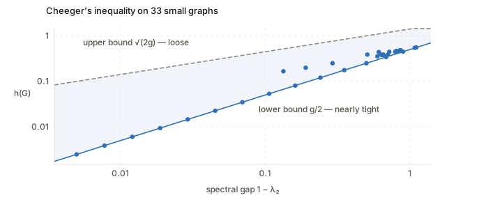
Why this matters for the papers. The loose direction is the one HaoChen et al. need. They have a combinatorial assumption (\rho_m large) and want a spectral conclusion, so they pay the square. That is exactly why Theorem 3.7 reads \tilde O(\alpha/\rho_{\lfloor k/2\rfloor}^2) with \rho squared: the square is not a statement about data, it is the price of the rounding argument. If someone proves a tighter higher-order Cheeger inequality, that exponent improves for free.
Higher-order Cheeger
Cheeger bipartitions. For m parts, the relevant statement (Lee–Oveis Gharan–Trevisan) is
\frac{1 - \lambda_m}{2} \;\lesssim\; \rho_m \;\lesssim\; O(m^2)\sqrt{1 - \lambda_m},
where \rho_m is the sparsest m-partition. This is what actually underwrites HaoChen et al.’s use of \rho_m: many eigenvalues near 1 \Leftrightarrow the graph splits into many weakly-connected pieces. It is the rigorous version of “count the eigenvalues near 1 to count the clusters”, and it is why raising the feature dimension k — which lets the analysis invoke a larger m, hence a larger \rho_m — improves the bound.
Eckart–Young–Mirsky
Not an inequality but an exact optimality statement, and load-bearing enough to belong here. The best rank-k approximation of M in Frobenius (or spectral) norm is its truncated SVD:
\min_{\operatorname{rank}(F) \le k} \lVert M - F\rVert_F^2 = \sum_{i > k}\sigma_i^2 .
Applied to M = \bar A and F = FF^\top, this is what turns the spectral contrastive loss from “a loss that vaguely encourages spreading out” into “an objective whose minimiser is exactly the top-k eigenvectors, up to a right rotation”. The residual \sum_{i>k}\lambda_i^2 is why the eigenvalues beyond k — the ones \lambda_{k+1} tracks — are what governs quality.
Weyl’s inequality and Cauchy interlacing
Weyl: for symmetric M, E, every eigenvalue moves by at most the perturbation’s norm:
\lvert \lambda_i(M + E) - \lambda_i(M)\rvert \le \lVert E\rVert_2 .
Crude but unconditional, and the first thing to reach for when a matrix is perturbed. It is what licenses Zhang et al.’s claim that adding \epsilon W to their idealised adjacency matrix does not destroy the spectral structure, provided \epsilon\lVert W\rVert_2 stays well below the gap between the class modes and the bulk.
Cauchy interlacing: deleting a row and column of a symmetric matrix interlaces the eigenvalues, \lambda_{i+1}(M) \le \lambda_i(M') \le \lambda_i(M). The reason removing data points cannot move the spectrum arbitrarily — background for any “what if we delete examples” argument.
Davis–Kahan
Weyl controls eigenvalues; Davis–Kahan controls eigenvectors:
\sin\Theta\big(\text{span}_k(M), \text{span}_k(M+E)\big) \lesssim \frac{\lVert E\rVert_2}{\text{gap}} .
The subspace moves in proportion to the perturbation divided by the eigenvalue gap around the cut. If the eigenvalues at the truncation boundary are nearly tied, the top-k subspace is ill-determined and an arbitrarily small perturbation can rotate it a lot.
This is precisely the shape of HaoChen et al.’s Theorem 4.2, whose penalty term is k\epsilon/\Delta with \Delta = \lambda_{\lfloor 3k/4\rfloor} - \lambda_k. The moral: any result that learns a subspace by truncating a spectrum must carry a gap condition somewhere, and if the spectrum has a long flat bulk — which is exactly what both the toy graph in the HaoChen notes and Zhang et al.’s construction exhibit — that term is the one to worry about.
Wigner’s semicircle law
For a symmetric N \times N matrix with i.i.d. mean-zero unit-variance entries, the eigenvalues of W/\sqrt N converge to the semicircle density on [-2, 2]:
p(x) = \frac{1}{2\pi}\sqrt{4 - x^2}.
Random noise has a predictable, compactly supported spectrum — so a perturbed matrix looks like the original spikes plus a semicircular bulk of width O(\epsilon\sqrt N). This is why Zhang et al.’s relaxation is analysable rather than hopeless, and where the Kepler equation in their Theorem B.4 comes from: solving for a quantile of the semicircle CDF gives an equation of exactly the form \tfrac{1}{2}x\sqrt{4-x^2} + 2\arcsin(x/2) = c.
It is also the practical lesson for reading any real spectrum: a bulk is not signal. Only eigenvalues separated from the bulk carry structure.
4. Limits and rates
Concentration of measure on the sphere
A 1-Lipschitz function on S^{d-1} with uniform measure concentrates around its mean with sub-gaussian tails of scale 1/\sqrt d:
\Pr\big[\lvert F(u) - \mathbb{E}F\rvert \ge t\big] \le 2e^{-cdt^2}.
In particular each coordinate of a uniform u is sub-gaussian with parameter O(1/\sqrt d) — the fact that supplies the constant in Betser et al.’s Lemma 1. High-dimensional spheres are strange: almost all the measure sits near any equator, which is the same phenomenon as the thin shell effect (Betser’s Assumption 2, and the r^{d-1}e^{-\lambda r^2} radial law), where a high-dimensional Gaussian’s mass concentrates on a sphere of relative width O(1/\sqrt d).
Maxwell–Poincaré spherical CLT, with a rate
For U_d uniform on S^{d-1} and fixed k:
\sqrt d\,(U_{d,1},\dots,U_{d,k}) \Rightarrow \mathcal{N}(0, I_k), \qquad d_{\mathrm{TV}} \le \frac{2(k+3)}{d-k-3} \quad (1 \le k \le d-4).
The sphere is Gaussian in high dimension, viewed through any fixed low-dimensional window. The explicit Diaconis–Freedman rate is what makes Betser et al.’s asymptotic statement useful at finite d: O(1/d), so d = 128 already gives total variation \lesssim 0.05 for small k. Worth having a rate rather than a bare limit — an asymptotic claim with no rate cannot be checked against an experiment.
Slutsky’s theorem
If X_n \Rightarrow X in distribution and Y_n \to c in probability, then Y_n X_n \Rightarrow cX. Mundane, and exactly the glue Betser et al.’s Proposition 2 needs: \sqrt d\,z_k = r\cdot(\sqrt d\,u_k), with the direction converging in distribution and the radius converging in probability to r_0, gives \mathcal{N}(0, r_0^2 I_k).
The condition worth noticing: Y_n must converge to a constant. If the radius kept a non-degenerate distribution, the limit would be a scale mixture of Gaussians — heavy-tailed, and rejected by exactly the normality tests those papers run. The thin-shell assumption is not decoration; without it the conclusion is false.
Berry–Esseen
\sup_t \big\lvert \Pr[\bar S_n \le t] - \Phi(t) \big\rvert \le \frac{C\rho_3}{\sigma^3\sqrt n}.
The CLT with a rate: O(n^{-1/2}), given a third moment. The generic answer to “the limit is Gaussian, but how far off am I at finite n?”, and the source of the O(N^{-1/2}) figure in Betser et al.’s discussion of finite batch sizes.
Patterns worth internalising
- Every concentration bound is Markov in disguise, applied to X, to (X-\mu)^2, or to e^{\lambda X}. If you remember only one inequality, remember Markov.
- Square roots mark rounding arguments. Cheeger’s \sqrt{2g} and Pinsker’s \sqrt{\mathrm{KL}/2} both appear when converting a continuous/spectral object back into a discrete decision. That is why HaoChen et al.’s bound has \rho^2 — the square is the cost of the conversion, not a property of the data.
- A variational formula is a lower-bound machine. Donsker–Varadhan turns “evaluate this divergence” into “guess a good test function”, which is almost always easier.
- Gaps in the denominator mean identifiability. Whenever a bound divides by an eigenvalue gap (Davis–Kahan, HaoChen Thm. 4.2), the real content is that the object being estimated must be well-separated to be recoverable at all.
- Chain rules buy free dimensions. If your objective is blind to part of a decomposition, a chain rule lets you solve that part exactly and shrink the problem.
- Dimension is sometimes an ally. Concentration on the sphere, thin shells, and the (d-1) factor in Betser et al.’s Lemma 1 all improve with dimension. The curse of dimensionality has a blessing attached.
Sources
Standard references rather than the papers themselves:
- Roman Vershynin, High-Dimensional Probability (2018) — sub-gaussian tails, concentration on the sphere, Davis–Kahan, Wigner. The single best starting point.
- Fan Chung, Spectral Graph Theory (1997) — Cheeger, the normalised Laplacian, conductance.
- Lee, Oveis Gharan & Trevisan, Multiway spectral partitioning and higher-order Cheeger inequalities (JACM 2014) — the \rho_m \leftrightarrow \lambda_m statement.
- Boucheron, Lugosi & Massart, Concentration Inequalities (2013) — McDiarmid, bounded differences, the whole ladder.
- Dupuis & Ellis, A Weak Convergence Approach to the Theory of Large Deviations (2011) — Donsker–Varadhan and the KL chain rule, as cited by both contrastive papers.
- Diaconis & Freedman, A dozen de Finetti-style results in search of a theory (1987) — the spherical CLT rate.