On the Importance of Gaussianizing Representations
Links
- arXiv:2505.00685: preprint of the ICML 2025 paper (PMLR 267). Code at DanielEftekhari/normality-normalization.
- Interactive companion: Eq 3 on the number line, a batch you can Gaussianize while watching the NLL and its Newton step, and Lemma B.1 as two scatter plots with sliders.
- Gaussianity in practice: the topic page cites this paper as reference [1], the one that Gaussianizes deliberately rather than assuming it.
- Betser 2026, InfoNCE induces Gaussian: the other direction. Contrastive training produces Gaussian features without being asked to.
- Runnable
code: checks every derivative in Appendices C–D against
finite differences (including the h<0 branch the paper skips), compares one
Newton step with the exact minimiser, and puts numbers on Lemma B.1.
make verifyruns it.
In one paragraph
BatchNorm, LayerNorm and friends fix the first two moments of each unit’s pre-activations but say nothing about the shape of the distribution. This paper argues the shape should be Gaussian, for information-theoretic reasons: a Gaussian carries the most information for a given variance, is the worst-case noise to be robust against, and is the one joint distribution where “uncorrelated” already means “independent”. It then builds a drop-in layer, normality normalization, that does four things: standardise as usual; estimate a Yeo–Johnson power transform exponent \hat\lambda with a single closed-form Newton step; apply the transform to Gaussianize each unit; and during training add Gaussian noise scaled by the batch’s mean absolute deviation. There are no new learned parameters. It beats the corresponding plain normalization layer across ResNets, WideResNets and ViTs (e.g. ImageNet top-1 with a ViT: 71.5 → 75.3), and Q–Q plots confirm the features stay Gaussian through training where BatchNorm’s drift away. The theory motivates the method but does not prove it works. The appendices contain one lemma (B.1) and two calculus derivations (C, D), all of which check out, with small caveats.
The spine of the argument
- Gaussian is special (§2): best signal, worst noise (Theorem 2.1); maximum entropy for a given variance; and for jointly Gaussian variables, uncorrelated ⇔ independent (Lemma B.1).
- So encourage Gaussian activations and train with Gaussian noise. Noise acts as a regulariser, and the Gaussian is the distribution that tolerates the most noise for the information it carries.
- Tool: the power transform (§3, Eq 3). It is a one-parameter monotone family, and its exponent is chosen by maximum likelihood (Eq 4, derived in Appendix C).
- Make it cheap (§4.1, Appendix D): Taylor-expand the NLL around \lambda=1 (identity) and take one Newton step. After standardisation the step needs only three batch averages.
- Add scaled Gaussian noise (§4.2), train only.
- Evidence (§5): accuracy across models, datasets, widths, depths and batch sizes; Q–Q normality through depth; ablations showing both the transform and the noise matter.
Setup and notation
| Symbol | Meaning |
|---|---|
| u_i, i=1..N | one channel’s raw pre-activations over the normalisation set (N=BHW for BatchNorm on conv layers) |
| h_i=(u_i-\hat\mu)/\sqrt{\hat\sigma^2+\epsilon} | the usual standardised value, so mean 0 and variance 1 |
| \psi(h;\lambda) | Yeo–Johnson power transform (Eq 3) |
| \lambda, \hat\lambda | transform exponent; its one-step Newton estimate (Eq 5) |
| x_i=\psi(h_i;\hat\lambda) | the Gaussianized value |
| \mathcal L(\boldsymbol h;\lambda) | profile negative log-likelihood of \lambda (Eqs 4, 13) |
| \mathcal L', \mathcal L'' | derivatives in \lambda, evaluated at \lambda=1 |
| \xi, s, z_i | noise factor (hyperparameter, 0.4 for ResNets, 1.0 for ViTs); scale s=\frac1N\sum\lvert x_i-\bar x\rvert (gradient-detached); z_i\sim\mathcal N(0,1) |
| y_i=x_i+z_i\,\xi\,s | noisy output (training only) |
| v_i=\gamma y_i+\beta | the usual learned affine step |
| I(X;Y), h(X) | mutual information; differential entropy |
§2 Motivation, in plain terms
Theorem 2.1: the mutual information game
Two players share an additive channel Y=X+Z. The signal X wants Y to reveal as much as possible about X (maximise I(X;X+Z)). The noise Z wants to hide X (minimise it). Each player may use any distribution with a given mean and variance. The theorem says both players should choose a Gaussian:
I(X;X+Z^*)\;\le\;I(X^*;X^*+Z^*)\;\le\;I(X^*;X^*+Z).
Read it left to right. Against Gaussian noise Z^*, no signal beats a Gaussian signal. For a Gaussian signal X^*, no noise hurts more than Gaussian noise. So (X^*,Z^*) is a saddle point and neither side gains by deviating (Eq 2).
Where each inequality comes from, since the paper’s one-line proof is terse:
- Left. I(X;X+Z^*)=h(X+Z^*)-h(Z^*). Only the first term depends on X, and X+Z^* has variance \sigma_x^2+\sigma_z^2 however X is distributed. The Gaussian has the largest entropy for that variance, so X+Z^* is best off being Gaussian, which happens when X is. This is maximum entropy.
- Right. I(X^*;X^*+Z)=h(X^*+Z)-h(Z). The entropy power inequality e^{2h(X^*+Z)}\ge e^{2h(X^*)}+e^{2h(Z)} lower-bounds it by \tfrac12\log\!\big(1+2\pi e\sigma_x^2/e^{2h(Z)}\big). Maximum entropy (e^{2h(Z)}\le2\pi e\sigma_z^2) then gives \tfrac12\log(1+\sigma_x^2/\sigma_z^2), the all-Gaussian value.
(The paper attributes EPI to the first inequality and maximum entropy to the second. As far as I can tell it’s the other way round, with the second needing both. The theorem itself is standard; see Cover & Thomas, ch. 9.)
How it’s used. Two heuristics: (i) if you’re going to inject noise as a regulariser, Gaussian noise is the hardest to be robust to, so it regularises most; (ii) Gaussian activations are the ones that keep the most information under a given amount of noise. Neither is a theorem about networks. It’s an analogy with each layer treated as a noisy channel.
Maximum entropy
For a fixed variance, the Gaussian has the largest differential entropy, h=\tfrac12\log(2\pi e\sigma^2). Since the normalisation layer already fixes the variance, a Gaussian unit is the one that “uses” that variance budget most fully.
Independence (this is where Lemma B.1 comes in)
For Gaussian variables, uncorrelated means independent. That is true only for jointly Gaussian variables, and the subtlety matters for this paper; see the Lemma B.1 section below.
§3 The power transform (Eq 3)
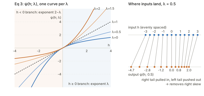
\psi(h;\lambda)=\begin{cases} \frac1\lambda\big((1+h)^\lambda-1\big), & h\ge0,\ \lambda\ne0\\[2pt] \log(1+h), & h\ge0,\ \lambda=0\\[2pt] \frac{-1}{2-\lambda}\big((1-h)^{2-\lambda}-1\big), & h<0,\ \lambda\ne2\\[2pt] -\log(1-h), & h<0,\ \lambda=2 \end{cases}
How to read it, one idea at a time:
- Right half (h\ge0) is the classic Box–Cox transform applied to 1+h. At \lambda=1 it’s h itself. At \lambda=0 it’s \log(1+h): the limit of (a^\lambda-1)/\lambda as \lambda\to0 is \log a, which is why that case is listed separately. For \lambda<1 it grows slower than linear and pulls big positives in.
- Left half (h<0) is the right half mirrored (h\mapsto-h, output negated) with exponent 2-\lambda instead of \lambda. So a \lambda that compresses the right tail (\lambda<1, hence 2-\lambda>1) stretches the left tail. Both effects push a right-skewed batch towards symmetry. This mirroring is Yeo & Johnson’s (2000) fix for Box–Cox only accepting positive inputs.
- Slope 1 at the origin for every \lambda. \partial\psi/\partial h=(1+h)^{\lambda-1} on the right and (1-h)^{1-\lambda} on the left, both 1 at h=0. So the transform leaves the bulk of a standardised batch almost alone and only bends the tails.
- Monotone. Both slopes are positive, so values are never reordered. The CDF argument in Appendix C relies on this.
- Limits of the family. One parameter, monotone, slope pinned at 0: it can remove skew but not symmetric heavy tails or multimodality. The code measures this: for a Student-t (5 dof) batch, \hat\lambda=0.96 and nothing changes; for a lognormal batch the skew falls from 1.34 to 0.15.
The interactive page lets you slide \lambda and watch the number line bend, then Gaussianize a batch of your choice.
§4 The layer (Algorithm 1)
Per channel, per minibatch:
- Standardise: h_i=(u_i-\hat\mu)/\sqrt{\hat\sigma^2+\epsilon}, exactly BatchNorm (or Layer/Instance/Group norm, depending on which axes are pooled).
- Estimate \hat\lambda with one Newton step (Eq 5): \hat\lambda=1-\mathcal L'(\boldsymbol h;1)/\mathcal L''(\boldsymbol h;1).
- Transform: x_i=\psi(h_i;\hat\lambda).
- Noise (training only): y_i=x_i+z_i\,\xi\,s with s=\frac1N\sum_i|x_i-\bar x|, computed with gradient tracking off. s is the mean absolute deviation, a robust spread estimate. For a standard-normal channel s=\sqrt{2/\pi}\approx0.80 (checked in code), so the noise standard deviation is about 0.8\,\xi.
- Affine: v_i=\gamma y_i+\beta.
At test time, a running average of \hat\lambda is kept alongside the running mean and variance, exactly as BatchNorm does for \mu,\sigma^2. No noise is added at test time.
Why standardise before transforming? Three reasons, one of them not stated in the paper. (i) It makes \hat\mu(1)=0 and \hat\sigma^2(1)=1, which is what collapses Appendix D to a few averages. (ii) Numerical stability. (iii) Yeo–Johnson isn’t scale-invariant: \psi(ch;\lambda) is not a rescaled \psi(h;\lambda). Fixing the scale first makes \lambda mean the same thing in every channel.
Why noise after the transform and additive? The paper’s argument (§5.6) is that dropout’s multiplicative noise enters the backward pass through the activations, while additive noise with a detached scale doesn’t change the gradients’ form. Fig 7 shows it beating Gaussian dropout at every retention rate tried, and beating unscaled noise with s fixed at \sqrt{2/\pi}. This is an empirical result, not a derived one.
Appendix C: deriving the NLL (Eqs 4 and 13)
What we want. A \lambda such that the transformed batch x_i=\psi(h_i;\lambda) looks like draws from some \mathcal N(\mu,\sigma^2). Maximum likelihood turns that into an equation: write down the density that the model “\psi(H;\lambda) is Gaussian” assigns to the observed h_i, and choose \lambda (and \mu,\sigma^2) to make it largest.
Step 1: the density of H (Eqs 9–10). The model is about X=\psi(H), but the data are values of H, so we need H’s density. Because \psi is increasing, “H\le h” is the same event as “X\le\psi(h)”:
F_H(h)=P(H\le h)=P\big(X\le\psi(h;\lambda)\big)=F_X\big(\psi(h;\lambda)\big).
Differentiate in h with the chain rule:
f_H(h)=f_X\big(\psi(h;\lambda)\big)\cdot\frac{\partial\psi}{\partial h}=f_X\big(\psi(h;\lambda)\big)\cdot(1+h)^{\lambda-1}\qquad(h\ge0).
This is the change-of-variables formula, the same one behind normalising flows. The extra factor \partial\psi/\partial h is the Jacobian: how much \psi stretches the axis near h. Where \psi squashes (slope below 1), a lot of H-probability lands in a little X-space, and the Jacobian accounts for that.
Step 2: the NLL (Eq 11). Average -\log f_H(h_i) over the batch, with f_X the \mathcal N(\mu,\sigma^2) density:
\mathcal L=\tfrac12\log(2\pi)+\tfrac12\log\sigma^2+\frac{1}{2N\sigma^2}\sum_i(x_i-\mu)^2-\frac{\lambda-1}{N}\sum_i\log(1+h_i).
The last term is the log-Jacobian, \log(1+h)^{\lambda-1}=(\lambda-1)\log(1+h).
Step 3: profile out \mu and \sigma^2 (Eqs 12–13). For fixed \lambda the best \mu,\sigma^2 are the sample mean and variance of the x_i (the usual Gaussian MLE). Substituting them makes the third term exactly \tfrac12:
\boxed{\ \mathcal L(\boldsymbol h;\lambda)=\tfrac12\big(\log(2\pi)+1\big)+\tfrac12\log\hat\sigma^2(\lambda)-\frac{\lambda-1}{N}\sum_i\log(1+h_i)\ }
This is Eq 13 (= Eq 4). “Profile” just means \mu and \sigma^2 have been optimised away, so it’s a function of \lambda alone.
Reading Eq 13 as a tug of war. The variance term \tfrac12\log\hat\sigma^2(\lambda) rewards any \lambda that shrinks the transformed batch. The Jacobian term charges for exactly that shrinking. Without it, the “most Gaussian-looking” answer would be whichever \lambda squashes hardest. The minimum balances the two, and the interactive page plots both parts separately.
The h<0 half, which the paper leaves to “symmetry”. It matters, because standardised h is negative about half the time. On the left branch \partial\psi/\partial h=(1-h)^{1-\lambda}, whose log is (1-\lambda)\log(1-h). Both branches together give a single term:
-\frac{\lambda-1}{N}\sum_i\operatorname{sign}(h_i)\,\log(1+|h_i|).
This is the standard Yeo–Johnson log-likelihood. The code uses it, and its finite-difference derivatives match the analytic ones below to five decimals.
Why the result is just the exact MLE. The profile NLL is exact, with no approximation yet. Approximation only enters in Appendix D.
Appendix D: one Newton step for \hat\lambda (Eqs 5, 14–21)
Why not just minimise Eq 13? There’s no closed form for \partial\mathcal L/\partial\lambda=0, and running an iterative solver inside every normalisation layer, every step, is expensive and adds a step-size hyperparameter. So the paper replaces \mathcal L by its second-order Taylor expansion around \lambda_0=1 (Eq 14),
\mathcal L_2(\lambda)=\mathcal L(1)+(\lambda-1)\,\mathcal L'(1)+\tfrac12(\lambda-1)^2\,\mathcal L''(1),
and minimises the parabola exactly: set \mathcal L_2'(\lambda)=0 to get Eq 5, \hat\lambda=1-\mathcal L'(1)/\mathcal L''(1). That is one step of Newton’s method started at \lambda=1. Why expand at 1: it’s the identity, so if the data are already Gaussian, \mathcal L'(1)\approx0 and \hat\lambda\approx1 leaves them alone. It’s also the “no preference” point between compressing and stretching.
The derivatives (Eq 15). Only two terms of Eq 13 depend on \lambda:
\mathcal L'=\frac{\partial_\lambda\hat\sigma^2}{2\hat\sigma^2}-\frac1N\sum_i\log(1+h_i),\qquad \mathcal L''=-\frac{(\partial_\lambda\hat\sigma^2)^2}{2\hat\sigma^4}+\frac{\partial^2_\lambda\hat\sigma^2}{2\hat\sigma^2}.
These are just derivatives of \tfrac12\log(\cdot) and of a linear function of \lambda. (Eq 15’s first line prints \tfrac12\log(2\pi+1); it should be \tfrac12(\log 2\pi+1), as in Eq 13. It is a constant and doesn’t affect \hat\lambda.)
Derivatives of the variance (Eqs 16–21). With \hat\sigma^2(\lambda)=\frac1N\sum(\psi_i-\hat\mu)^2 and \psi_i=\psi(h_i;\lambda), the paper differentiates term by term. One simplification it doesn’t use: since \sum_i(\psi_i-\hat\mu)=0 always, every term multiplying \partial_\lambda\hat\mu or \partial^2_\lambda\hat\mu is zero:
\partial_\lambda\hat\sigma^2=\frac2N\sum_i(\psi_i-\hat\mu)\,\partial_\lambda\psi_i,\qquad \partial^2_\lambda\hat\sigma^2=\frac2N\sum_i\Big[(\psi_i-\hat\mu)\,\partial^2_\lambda\psi_i+\big(\partial_\lambda\psi_i-\overline{\partial_\lambda\psi}\big)^2\Big].
Evaluate at \lambda=1. Now three facts collapse everything:
- \psi(h;1)=h on both branches (identity);
- the batch is already standardised: \hat\mu(1)=0, \hat\sigma^2(1)=1;
- the \lambda-derivatives of \psi at \lambda=1 have closed forms. With t=|h|:
\partial_\lambda\psi\big|_{1}=(1+t)\log(1+t)-t\quad\text{(even in }h\text{)},\qquad \partial^2_\lambda\psi\big|_{1}=\operatorname{sign}(h)\Big[(1+t)\log^2(1+t)-2\big((1+t)\log(1+t)-t\big)\Big]\quad\text{(odd)}.
For h\ge0 these are Eqs 18 and 21. The h<0 versions aren’t in the paper. Derived here: on that branch the exponent is m=2-\lambda, so one \lambda-derivative flips sign twice (even), and the second derivative flips once (odd). The code checks both against finite differences (max error 3\times10^{-8}).
Writing a_i=\partial_\lambda\psi(h_i;1) and b_i=\partial^2_\lambda\psi(h_i;1), the whole Newton step is three batch averages:
\mathcal L'(1)=\overline{h\,a}-\overline{\operatorname{sign}(h)\log(1+|h|)},\qquad \mathcal L''(1)=-2\,\big(\overline{h\,a}\big)^2+\overline{h\,b}+\operatorname{Var}(a),\qquad \hat\lambda=1-\frac{\mathcal L'(1)}{\mathcal L''(1)}.
The code confirms this matches a literal transcription of Eqs 15–21 (difference 9\times10^{-6}, from the \epsilon in the standardisation).
Intuition for the sign. a\approx h^2/2 for small |h|, so \overline{h\,a}\approx\tfrac12\overline{h^3}, which is half the skewness. The log term is odd and vanishes for symmetric data. So right skew ⇒ \mathcal L'(1)>0 ⇒ \hat\lambda<1 ⇒ compress the right tail, which is the correct move. Numerically, for mild skew, 1-\hat\lambda\approx0.5\times skewness (the code measures a ratio of 0.48–0.53 on lognormal batches).
How good is one step? It’s exact when \mathcal L is quadratic, and the paper’s Fig 13 shows real ResNet18 activations are in that regime. Off-regime it degrades (code, N=4096):
| batch | skew | Newton \hat\lambda | exact minimiser | skew after Newton |
|---|---|---|---|---|
| Gaussian | −0.05 | 1.02 | 1.02 | −0.01 |
| Student-t, 5 dof | 0.20 | 0.96 | 0.96 | 0.04 |
| lognormal \sigma=0.4 | 1.34 | 0.47 | 0.40 | 0.15 |
| left-skew -\text{Gamma}(3) | −1.12 | 1.57 | 1.62 | −0.14 |
| Gamma(2) (ReLU-like) | 1.53 | 0.33 | 0.22 | 0.25 |
| lognormal \sigma=0.8 | 3.00 | 0.10 | −0.32 | 0.64 |
Every case moves in the right direction and cuts the skew a lot, but for heavily skewed channels one step undershoots. That’s a deliberate trade for a closed form. The paper’s α-ablation (Fig 8, scaling the step by \alpha\le1) suggests the full step is already the best of the step sizes tried. Nobody checked \alpha>1 or a second step.
Appendix B: Lemma B.1, Gaussian joints minimise mutual information
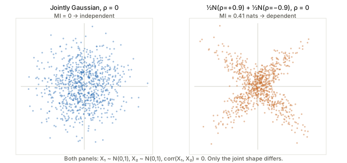
Statement, with the hidden assumption made explicit. Let X_1\sim\mathcal N(\mu_1,\sigma_1^2) and X_2\sim\mathcal N(\mu_2,\sigma_2^2), with correlation \rho. Among all joint distributions with these marginals and this correlation, the jointly Gaussian one has the smallest mutual information, and that minimum is
I(X_1;X_2)=-\tfrac12\log(1-\rho^2).
(The lemma as printed fixes only the marginals, but the proof needs the covariance fixed too: the maximum-entropy step compares distributions with the same covariance. §2.3’s wording, “for any given degree of correlation”, shows this is what is meant.)
The proof, line by line (Eq 8). Call the Gaussian joint f and any competitor g with the same marginals and \rho.
- I_g(X_1;X_2)=h_g(X_1)+h_g(X_2)-h_g(X_1,X_2). This is the definition: information = what the parts’ uncertainty adds up to, minus the uncertainty of the pair.
- =h_f(X_1)+h_f(X_2)-h_g(X_1,X_2). The marginals are the same normal distributions under f and g, so their entropies agree.
- \ge h_f(X_1)+h_f(X_2)-h_f(X_1,X_2). For a fixed covariance matrix, the Gaussian has the largest joint entropy, so h_g(X_1,X_2)\le h_f(X_1,X_2). Subtracting something larger gives something smaller.
- =I_f(X_1;X_2), then plug in the entropies: h(\mathcal N(\mu,\sigma^2))=\tfrac12\log(2\pi e\sigma^2), and the bivariate normal has h=\tfrac12\log\big((2\pi e)^2\det\Sigma\big) with \det\Sigma=\sigma_1^2\sigma_2^2(1-\rho^2). Everything cancels except -\tfrac12\log(1-\rho^2).
In words: once the marginals and the correlation are fixed, the only thing left to vary is the joint entropy. The Gaussian maximises it, so it minimises the information shared. In a Gaussian, correlation is the only dependence. Any other joint with the same \rho hides extra dependence that \rho doesn’t see.
The corollary. Jointly Gaussian and \rho=0 ⇒ I=0 ⇒ independent.
What the lemma does not say, which is where the figure above comes in. It does not say that normal marginals plus \rho=0 give independence. The right panel is an equal mixture of bivariate normals with correlations \pm0.9. Both coordinates are exactly \mathcal N(0,1) and uncorrelated, but the mutual information is 0.41 nats (code). Other rows from the code show the lemma’s inequality directly:
| joint with \mathcal N(0,1) marginals | \rho | MI (nats) | Gaussian MI at the same \rho |
|---|---|---|---|
| ½N(+0.6) + ½N(−0.6) | 0.00 | 0.053 | 0 |
| ½N(+0.9) + ½N(−0.9) | 0.00 | 0.408 | 0 |
| ½N(+0.9) + ½N(+0.1) | 0.50 | 0.219 | 0.144 |
| ½N(+0.8) + ½N(+0.4) | 0.60 | 0.233 | 0.223 |
A consequence for the method. Mutual information is unchanged by any invertible function applied to each variable separately: I(\psi_1(X_1);\psi_2(X_2))=I(X_1;X_2). The power transform is exactly such a per-unit map. So the transform step by itself cannot make two units more independent. It changes their marginals and their Pearson correlation (the code’s example: \rho=0.6\to0.46 after X_2\mapsto e^{X_2}, with MI fixed at 0.223), but not the dependence. The independence gains in Fig 12 (lower adjusted MI between channel pairs) must therefore come from training reacting to the layer. The paper’s phrase “increased unit-wise normality also lends itself to increased joint normality” is a hope that Fig 12 supports empirically, not something Lemma B.1 delivers.
Results, briefly
- Accuracy. ViT + LayerNormalNorm vs LayerNorm (Table 1): CIFAR-100 66.4 → 70.1, Food-101 73.3 → 79.1, ImageNet top-1 71.5 → 75.3. ResNets + BatchNormalNorm vs BatchNorm without augmentation (Table 2): CIFAR-100 62.0 → 65.8, STL-10 58.8 → 63.9. It also helps Group/Instance norm (Fig 1) and decorrelated BN (Table 3). Six seeds each; standard errors are small next to the gaps.
- Robust across configurations. The gap is largest for narrow WideResNets (Fig 2), which the authors connect to narrow nets being furthest from the infinite-width Gaussian-process limit. It persists across depth (Fig 3) and batch size (Fig 4).
- It does Gaussianize. Q–Q R^2 stays at about 0.95–0.99 in every layer with BNN, while BatchNorm’s swings between 0.4 and 0.95 (Fig 6). At initialisation both are Gaussian (Fig 11); BN drifts away during training.
- Both parts matter (Fig 9): transform without noise beats BN, and adding the noise helps further. Fig 8: stronger Gaussianization (larger \alpha) means higher accuracy.
- Noise robustness at test time (Table 4): the relative change in a later layer’s output under injected noise is smaller with BNN in 29 of the 30 layer pairs, often by 2–5×.
- Cost: by eye from Fig 10, training is roughly 1.5–1.8× slower per sample than BatchNorm, and evaluation roughly 1.2–1.4× slower.
Questions and doubts
- The theory motivates but doesn’t explain. Theorem 2.1 is about one additive channel with moment constraints. A deep net is many coupled nonlinear “channels” whose weights adapt to the noise. The step from “Gaussian is the saddle point of the MI game” to “Gaussianized activations generalise better” is an analogy. The experiments carry the argument, not the lemmas.
- Lemma B.1 vs. what the method can do. As shown above, a per-unit transform leaves MI between units untouched. So the independence story is at best indirect. A cleaner test would measure MI between channel pairs before and after the transform in the same trained network (it should be identical) versus across networks trained with BN vs BNN (Fig 12’s comparison).
- Is it the shape or the regularisation? Yeo–Johnson with \lambda<1 also compresses outliers, which could help optimisation independently of Gaussianity (compare clipping or a robust scale). An ablation against a skew-agnostic squashing (e.g. a fixed \operatorname{sign}(h)\log(1+|h|)) would separate “Gaussian” from “bounded tails”.
- Only skew is corrected. Heavy symmetric tails and bimodality pass through untouched (code: t-distribution \hat\lambda=0.96). Yet the Q–Q plots are near-perfect, which suggests trained pre-activations are mostly skewed, not heavy-tailed. That’s plausible (post-ReLU inputs), but the paper doesn’t say so.
- “Convexity of the NLL”. §4.1 cites Yeo & Johnson (2000) for the NLL being convex in \lambda. What Yeo & Johnson prove, and what §6 restates, is convexity of \psi in \lambda (concavity for negative inputs). That isn’t the same thing. Fig 13 shows convex-looking curves, and the code found \mathcal L''(1)>0 on every batch tried. But nothing stops \mathcal L''(1)\le0 on a pathological batch, which would send the Newton step the wrong way. Whether the official code clamps \hat\lambda is worth checking.
- One step undershoots on strongly skewed channels (table above). Does a second Newton step, or \alpha>1 in Eq 6, help or hurt accuracy? The α-ablation stops at 1.
- \hat\lambda is a batch statistic. For LayerNorm on a ViT, N is the hidden size (768), fine. For small-batch BatchNorm on late conv layers, N=BHW can be small, and the third-moment-driven \hat\lambda will be noisy. Fig 4 shows small batches still help, but the variance of \hat\lambda itself isn’t reported.
- Typos/omissions in the appendix: Eq 15’s \tfrac12\log(2\pi+1); the h<0 branch of Eqs 10, 13, 18, 21 is left to “symmetry”, though half the inputs use it; the attributions of EPI and maximum entropy in Theorem 2.1’s proof look swapped. None of these change the results.
Takeaways
- Normalization layers can control shape, not just location and scale, and it’s cheap. One closed-form Newton step on three batch averages picks the power-transform exponent. No new learned parameters.
- Appendix C is the change-of-variables formula: NLL
= Gaussian fit to the transformed data
- a Jacobian charge for squashing. It’s the same bookkeeping as a normalising flow with one parameter.
- Appendix D is Newton’s method from the identity. After standardisation, \hat\lambda\approx1-\tfrac12\,\text{skewness} for mildly skewed channels. It’s accurate for the mild skew real activations show, and undershoots on strong skew.
- Lemma B.1 in one line: with the marginals and \rho fixed, the Gaussian joint has the most entropy and therefore the least shared information. Normal marginals alone don’t give “uncorrelated ⇒ independent”; the joint must be Gaussian. Per-unit transforms can’t change MI, so any independence benefit is indirect.
- Empirically strong and consistent across normalization types, architectures, widths, depths and batch sizes, at a 1.5–1.8× training-time cost. The theoretical motivation is best read as a reason to try Gaussian, not as the explanation for why it works.