Deep Learning versus Kernel Learning: an Empirical Study of Loss Landscape Geometry and the Time Evolution of the Neural Tangent Kernel
Links
- arXiv:2010.15110 —
preprint.
make fetchpulls the PDF from here. - Jacot et al. 2018 — the theory this paper measures against. Read that first.
- Runnable
code — kernel distance and velocity on a small network,
reproducing the transient.
make verifyruns it.
In one paragraph
Jacot proves the tangent kernel is constant in the infinite-width, small-learning-rate limit. Real networks are neither, so how do they differ and when? Fort et al. answer empirically, by measuring a dozen apparently unrelated quantities simultaneously — loss-landscape geometry, linear connectivity between independently trained copies, and the time evolution of a data-dependent NTK — and finding they all move together. The picture that emerges: a chaotic transient lasting two to three epochs during which the kernel moves fast and the network’s final basin is irreversibly decided, followed by a stable regime in which the kernel drifts slowly at constant speed. The theory describes the second phase well and is blind to the first — which is where the features are learned.
The spine of the argument
- Treat the NTK as a time-varying, data-dependent object and measure it, rather than assuming it constant.
- Detect when training makes an irreversible decision, using parent–child spawning plus a linear-interpolation error barrier.
- Observe that kernel velocity and error barrier collapse together, within 2–3 epochs.
- Ask when the kernel becomes useful: train fully to \tilde t, then linearise there. This isolates how much of the final performance is attributable to a learned kernel.
- Show that even at tiny learning rates, nonlinear training beats linearised training with a learned kernel during the early phase — so the early dynamics are irreducibly nonlinear.
Setup and notation
| Symbol | Meaning |
|---|---|
| J_w(x) \in \mathbb{R}^{K\times d} | Jacobian of the K logits w.r.t. the d parameters |
| \kappa_t(x,x') = J_t(x)J_t(x')^\top | the NTK, explicitly time-indexed and evaluated on data |
| \kappa_t(S) | the m\times m Gram matrix on a training subset S |
| S(w,w') | kernel distance between two kernels (below) |
| v(t) = S(w_t, w_{t+dt})/dt | kernel velocity; they use dt = 0.4 epochs |
| t_s | spawn time — when children are cloned off a parent |
| w_t^\alpha = \alpha w_t + (1-\alpha)w_t' | linear interpolation between two children |
| \tilde t | onset time of linearised training; \tilde t = 0 recovers the classic NTK |
| B_w(S) | binary ReLU activation pattern tensor, compared by Hamming distance |
Kernel distance
S(w,w') = 1 - \frac{\operatorname{Tr}(\kappa_w \kappa_{w'}^\top)} {\sqrt{\operatorname{Tr}(\kappa_w\kappa_w^\top)\operatorname{Tr}(\kappa_{w'}\kappa_{w'}^\top)}}
This is one minus the cosine similarity between the two Gram matrices viewed as flat vectors. Deliberately scale-invariant: the kernel’s overall magnitude drifts during training, and what they care about is which features it encodes, not how large it is. The cost of that choice is noted under doubts.
Parent–child spawning and the error barrier
Train a parent to t_s, clone it, train the children on independent minibatch sequences. Then measure whether the children ended up in the same basin, operationally:
\max_{\alpha\in[0,1]} \hat R_S(w_t^\alpha) - \tfrac12\big(\hat R_S(w_t) + \hat R_S(w_t')\big)
Zero barrier means the two are linearly connected through low loss, hence in one basin. So the earliest t_s at which children reliably end up with no barrier is the moment basin fate was sealed. That triple — spawn, interpolate, measure — is a genuinely clever instrument for detecting when training makes an irreversible choice, and it transfers well beyond NTK questions.
The data-dependent NTK
Train the full nonlinear network to time \tilde t, Taylor-expand there, and train linearly thereafter. Geometrically: walk along the curved function manifold to an intermediate point, then train only within that point’s tangent plane. Classic NTK is \tilde t = 0. This is the paper’s best idea, because it converts “does the kernel learn anything useful?” into a measurable quantity.
The core finding
A chaotic → stable transition completing within 2–3 epochs. During it:
- the error barrier between children collapses to zero — basin fate is decided;
- the kernel velocity collapses, then stabilises at a low but nonzero constant;
- these two curves are tightly correlated (their Fig. 7).
After the transient the kernel keeps moving, at constant speed, but the network can no longer change which basin it is in.
Reproduced
code/kernel_velocity.py measures the same two quantities
on a small MLP. The parametrisation matters and is worth stating
plainly: Jacot’s 1/\sqrt{n}
scaling deliberately suppresses kernel motion, so running this
measurement there shows almost nothing. Fort et al. study ordinary
He-initialised networks trained with ordinary SGD.
| config | v(epoch 1) | v(late) | ratio | % of total motion by epoch 3 |
|---|---|---|---|---|
| n=256, lr=0.002 | 0.0003 | 0.00002 | 16× | 52% |
| n=256, lr=0.02 | 0.0006 | 0.00004 | 14× | 42% |
| n=256, lr=0.08 | 0.0348 | 0.00049 | 71× | 62% |
| n=64, lr=0.02 | 0.0021 | 0.00018 | 12× | 45% |
| n=1024, lr=0.02 | 0.0258 | 0.00004 | 686× | 96% |
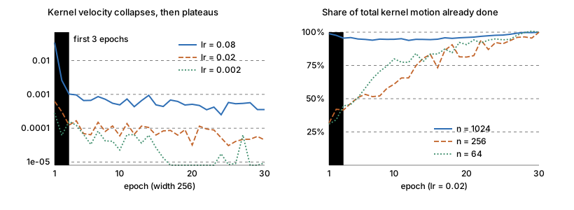
The n=1024 row states the tension with Jacot most sharply: 96% of the kernel’s total motion happens in the first three epochs, after which velocity falls to 4\times10^{-5} and it effectively freezes. The wide network does eventually behave as the theory says — but only after the interesting part is over.
The two results that matter most
Feature learning is real, fast, and front-loaded (their Fig. 8). Within \tilde t = 3–4 epochs the data-dependent NTK beats the initialisation kernel by a factor of 3 in error. By \tilde t = 30–90 epochs — 15% to 45% of training — it matches full network training.
Note this is two different clocks, and the paper is careful to keep them apart: basin fate is sealed by epoch 3, but the kernel needs 30–90 epochs to become as good as the full network. Kernel learning continues long after the chaotic phase ends, just more slowly.
The early phase is irreducibly nonlinear (their Fig. 9). Even at very low learning rate — the regime the NTK limit is supposed to describe — nonlinear training retains an advantage over linearised training with a learned kernel, during the early phase. And that advantage vanishes exactly when the error barrier does.
This is much sharper than “NTK fails at large learning rate”. It says you cannot rescue linearisation by handing it a better kernel: something happens in the first few epochs that no tangent-plane approximation captures, whichever tangent plane you choose.
What this does to the NTK picture
Read against the Jacot notes, the two fit together almost too neatly. Jacot proves the kernel is constant in the limit; Fort measures that at realistic width and learning rate it is very much not constant early, then becomes nearly constant with a small residual drift.
So the theory’s validity window opens right after basin fate is sealed. It describes the phase in which the network has stopped learning features, and is blind to the phase in which it learns them. That reframes “a constant kernel means no feature learning” from an abstract limitation into a measurable statement about when the approximation starts being true.
Questions and doubts
- “Correlated” is doing heavy lifting. The central claim is that many measures move together. That is suggestive but not causal: it could be one latent variable or several coincidentally-timed ones, and nothing here distinguishes those.
- “Chaotic” is used loosely. No Lyapunov exponent, no sensitivity measurement in the dynamical-systems sense. Operationally it means “sensitive to minibatch noise”, which is what spawning tests — reasonable, but the word imports connotations the measurements do not establish.
- Kernel distance is blind to spectral rescaling. \kappa \to c\kappa gives distance exactly 0. The invariance is deliberate, but it means a kernel whose conditioning changes dramatically while its direction holds registers as no movement, and some feature learning could hide there.
- No width sweep in the main analysis, which is striking for a paper about NTK — width is the parameter the theory is asymptotic in. Two architectures at fixed width. “NTK theory is a poor description at finite width” would be far stronger with a width axis showing the discrepancy shrink.
- 15%–45% is a wide range with no predictor. The data-dependent NTK result is the most actionable finding, but you cannot act on it without knowing \tilde t in advance, and nothing here predicts it.
- Cost is real and undiscussed. Repeatedly computing NTK Gram matrices over training is expensive; they subsample, and the error bars do not obviously account for it.
Takeaways
- The NTK is not constant, and the departure is concentrated in a two-to-three epoch window at the very start of training. Everything after that is close to the theory.
- Basin fate is sealed early — long before the loss has converged, and before the kernel has become useful. Two separate clocks, and conflating them is easy.
- Handing linearised training a better kernel does not rescue it during the early phase. The failure of NTK theory there is not about the kernel being random; it is about the dynamics being nonlinear.
- The most transferable contribution is an instrument, not a result: parent–child spawning plus a linear-interpolation error barrier is a cheap, general way to detect when training makes an irreversible decision. That applies to fine-tuning, curriculum design, and deciding which checkpoints are worth keeping.