HSIC: the Hilbert–Schmidt independence criterion
Links
- Interactive version: pick (or click in) a data set and watch correlation fail where HSIC succeeds; add polynomial features one degree at a time and see which cross-covariance lights up; hover over the two centred Gram matrices to see which pairs of samples agree; slide the kernel bandwidth from “blind” to “linear” and watch the permutation test respond; and compare two representations with CKA while rotating, stretching and warping one of them.
- Runnable
code: every number on this page, and the three figures
(
python3 hsic.py --figures).make verifyruns it. - Read first: the Gram matrix, especially §6 (centring, HGH) and §7 (kernels and the RBF bandwidth). HSIC is built from exactly those two pieces.
- Related foundations pages: four fundamental subspaces (the cross-covariance matrix X^\top Y), and the HGR maximal correlation section of inequalities and concentration (another “zero iff independent” measure, compared in §9 below).
- Primary references: A. Gretton, O. Bousquet, A. Smola & B. Schölkopf, Measuring Statistical Dependence with Hilbert–Schmidt Norms, ALT 2005 (the definition and the estimator); A. Gretton, K. Fukumizu, C. H. Teo, L. Song, B. Schölkopf & A. Smola, A Kernel Statistical Test of Independence, NeurIPS 2007 (the test); S. Kornblith, M. Norouzi, H. Lee & G. Hinton, Similarity of Neural Network Representations Revisited, ICML 2019 (CKA).
In one paragraph
Two variables are independent when learning one tells you nothing at all about the other. Correlation checks only one way of “telling”: whether y rises or falls along a straight line as x rises. HSIC checks every way at once, using nothing more than two Gram matrices. Build a table of how similar every pair of samples is in x (the matrix K) and another for y (the matrix L), centre both, and ask how well the two tables agree: \mathrm{HSIC}=\frac{1}{n^2}\sum_{ij}\tilde K_{ij}\tilde L_{ij}. If pairs that are unusually alike in x also tend to be unusually alike in y, the sum is large. With a plain dot product as the similarity, this is just the squared covariance. With a Gaussian similarity it is zero only when the variables are truly independent. The name describes the same number from the other side: it is the Hilbert–Schmidt norm (the Frobenius norm, for infinitely large matrices) of the table of covariances between every feature of x and every feature of y. A raw HSIC value means little on its own. It is judged against shuffled copies of the data, and normalising it gives CKA, the standard way to compare two networks’ representations.
1. The problem: “uncorrelated” is not “independent”
Independence in plain words. x and y are independent if the whole distribution of y (its average, its spread, its shape) is the same whatever value x takes. In symbols, p(x,y)=p(x)\,p(y): the probability of seeing a particular pair equals the probability of that x times the probability of that y, as if they were drawn by two separate coin-flips. Here p(x,y) is the joint distribution, the one that produced the pairs, and p(x), p(y) are the marginals, what you get by looking at one column of the data and ignoring the other.
What correlation checks. Five points on a parabola:
x=(-2,-1,0,1,2),\qquad y=x^2=(4,1,0,1,4).
The covariance is \operatorname{mean}(xy)-\operatorname{mean}(x)\operatorname{mean}(y)=\operatorname{mean}(x^3)-0\cdot 2=0, because the cubes cancel in pairs. So the correlation is exactly 0, and yet y is a function of x. Correlation only asks “does y go up when x goes up?”, and on a parabola it goes up on one side and down on the other, in exact balance.
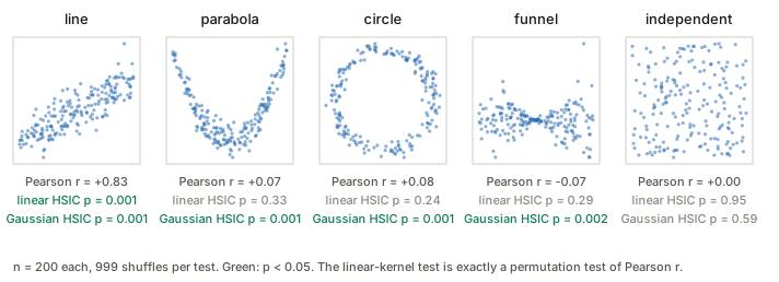
The funnel is the subtle one: y=x\cdot\varepsilon with \varepsilon standard normal noise. The average of y is 0 for every x, so no regression of y on x would find anything. Only the spread of y depends on x. That still counts as dependence.
2. Covariance is already a Gram-matrix formula
Centre each variable by subtracting its mean, \tilde x_i=x_i-\bar x and \tilde y_i=y_i-\bar y. With the \frac1n convention the covariance is \frac1n\sum_i\tilde x_i\tilde y_i. Square it and write the square as a double sum:
\operatorname{Cov}(x,y)^2=\frac{1}{n^2}\Big(\sum_i\tilde x_i\tilde y_i\Big)\Big(\sum_j\tilde x_j\tilde y_j\Big) =\frac{1}{n^2}\sum_{i,j}\underbrace{(\tilde x_i\tilde x_j)}_{\tilde K_{ij}}\;\underbrace{(\tilde y_i\tilde y_j)}_{\tilde L_{ij}} .
The two brackets are entries of Gram matrices: \tilde K=\tilde x\tilde x^\top holds the dot products of the centred x values (for numbers, a dot product is just a product) and \tilde L=\tilde y\tilde y^\top does the same for y. So squared covariance already measures how well two centred Gram matrices agree, entry by entry. That is HSIC with the linear kernel.
Vectors. Let x\in\mathbb R^p and y\in\mathbb R^q, stacked as rows of X (n\times p) and Y (n\times q). Now there are p\times q covariances, one for each coordinate of x against each coordinate of y. They form the cross-covariance matrix
C=\tfrac1n\tilde X^\top\tilde Y\quad(p\times q),
and the sum of the squares of all its entries is
\lVert C\rVert_F^2=\sum_{a,b}C_{ab}^2=\frac{1}{n^2}\operatorname{tr}\big(\tilde Y^\top\tilde X\tilde X^\top\tilde Y\big) =\frac{1}{n^2}\operatorname{tr}\big(\tilde K\tilde L\big),
using \lVert C\rVert_F^2=\operatorname{tr}(C^\top C) and the cyclic rule \operatorname{tr}(AB)=\operatorname{tr}(BA) to move \tilde Y to the end. Summing the squares of all covariances on the feature side (p\times q) and comparing Gram matrices on the sample side (n\times n) are the same computation, the dual view again.
A small case: the three points of the Gram matrix page, x_1=(1,0), x_2=(1,1), x_3=(0,2), with y=(1,3,2). Centring gives
\tilde X=\begin{bmatrix}\tfrac13&-1\\ \tfrac13&0\\ -\tfrac23&1\end{bmatrix},\qquad \tilde y=\begin{bmatrix}-1\\1\\0\end{bmatrix},\qquad C=\tfrac13\tilde X^\top\tilde y=\begin{bmatrix}0\\ \tfrac13\end{bmatrix}.
The first coordinate of x has no covariance with y and the second has covariance \frac13, so \mathrm{HSIC}=0^2+(\frac13)^2=\frac19\approx0.111, and \frac19\operatorname{tr}(\tilde K\tilde L) gives the same number.
Two remarks that will matter later. First, \lVert C\rVert_F^2 is the sum of the squared singular values of C. HSIC adds up the dependence along every direction, not only along the strongest one; §9 compares measures that keep only the strongest. Second, a shuffle test with the linear kernel is exactly a shuffle test of Pearson’s r: shuffling y changes neither \operatorname{Var}(x) nor \operatorname{Var}(y), so ranking shuffles by \operatorname{Cov}^2 ranks them by r^2. That is why Figure 1 needs only one “linear” row.
3. More features, more chances to catch dependence
Here is the key fact, in words. If x and y are independent, then no feature of x is correlated with any feature of y: \operatorname{Cov}(f(x),g(y))=0 for every pair of functions f,g. The converse also holds if you check a rich enough family of features: if every such covariance is zero, the variables are independent. So instead of one covariance, compute many.
Back to the five-point parabola, and give x two features instead of one: \varphi(x)=(x,\,x^2).
\operatorname{Cov}(x,y)=0,\qquad \operatorname{Cov}(x^2,y)=\operatorname{Var}(y)=2.8,
the second because x^2 is y. The sum of squared cross-covariances is 0^2+2.8^2=7.84. The dependence was invisible to the feature x and obvious to the feature x^2.
The kernel trick. In §2 the features only ever entered through dot products. With the features (x,x^2) the dot product between two samples is
k(x,x')=\varphi(x)\cdot\varphi(x')=x\,x'+x^2x'^2 .
Put this k into K, keep L=yy^\top, compute \frac{1}{n^2}\operatorname{tr}(\tilde K\tilde L), and out comes 7.84 again, without ever writing down the cross-covariance matrix. This is what makes it possible to use very many features, even infinitely many.
With the features (x,x^2,x^3) against (y,y^2,y^3), each kind of dependence lights up a different cell of the 3\times3 table of correlations between a feature of x and a feature of y:
- parabola: x^2 with y, because y is x^2.
- circle: x^2 with y^2, negatively, because x^2+y^2\approx1.
- funnel: x^2 with y^2, positively: big \lvert x\rvert means a big spread of y.
The funnel is the hardest of the three. Its y^2 has heavy tails, so the sample correlations that involve it are noisy, and cells that are exactly zero in the population by symmetry can read as small nonzero values in a sample. This matches the funnel’s weaker p-value in Figure 1. Widget 2 of the interactive page lets you raise the degree and watch cells appear.
The Gaussian kernel includes every degree. Expand the Gaussian (RBF) kernel for numbers:
e^{-(x-x')^2/2\sigma^2}=e^{-x^2/2\sigma^2}\,e^{-x'^2/2\sigma^2}\,e^{xx'/\sigma^2}, \qquad e^{xx'/\sigma^2}=\sum_{k=0}^{\infty}\frac{(xx')^k}{\sigma^{2k}\,k!}.
So k(x,x')=\sum_k\varphi_k(x)\varphi_k(x') with \varphi_k(x)=e^{-x^2/2\sigma^2}\,x^k/(\sigma^k\sqrt{k!}): one feature for every power of x, suitably weighted. The Gaussian kernel is the polynomial-feature idea with all degrees included at once, which is why it can catch any kind of dependence given enough data.
Decoding the name. Now each word has a concrete meaning:
- A Hilbert space is a vector space with a dot product that is allowed to have infinitely many coordinates, like the list of features \varphi_0(x),\varphi_1(x),\dots above.
- The one built from a kernel is its RKHS (reproducing kernel Hilbert space). Its coordinates are the kernel’s features, and “reproducing” means the dot product there is computed by k itself.
- The cross-covariance operator C_{xy} is the table of covariances between every feature of x and every feature of y: the matrix C of §2, but with infinitely many rows and columns.
- Its Hilbert–Schmidt norm is the square root of the sum of squares of all its entries. That is the Frobenius norm, carried over to such infinite tables, and it stays finite for the kernels used here.
So \mathrm{HSIC}=\lVert C_{xy}\rVert_{\mathrm{HS}}^2: the sum of squared covariances between every feature of x and every feature of y.
4. The estimator, symbol by symbol
\mathrm{HSIC}_b(X,Y)=\frac{1}{n^2}\operatorname{tr}(KHLH)=\frac{1}{n^2}\sum_{i,j}\tilde K_{ij}\tilde L_{ij}.
| Symbol | Read it as |
|---|---|
| n | number of paired samples (x_i,y_i) |
| K, K_{ij}=k(x_i,x_j) | how similar samples i and j are in x |
| L, L_{ij}=l(y_i,y_j) | how similar samples i and j are in y (the kernel l may differ from k) |
| H=I-\frac1n\mathbf 1\mathbf 1^\top | the centring matrix: subtracts means (Gram matrix §6) |
| \tilde K=HKH, \tilde L=HLH | the same similarities with row and column averages removed |
| \operatorname{tr} | the trace, the sum of the diagonal |
| subscript b | “biased”: its average is slightly above zero even for independent data (§7) |
The second form follows from H^2=H and the cyclic rule: \operatorname{tr}(KHLH)=\operatorname{tr}(HKH\cdot HLH)=\operatorname{tr}(\tilde K\tilde L), and for symmetric matrices \operatorname{tr}(\tilde K\tilde L)=\sum_{ij}\tilde K_{ij}\tilde L_{ij}. Gretton et al. (2005) divide by (n-1)^2 instead of n^2. That rescales the number and changes nothing in a test.
How to read it. \tilde K_{ij}>0 says “i and j are more alike in x than a typical pair is”. \tilde L_{ij}>0 says the same about y. Their product is positive when x and y agree about the pair (both say alike, or both say different) and negative when they disagree. HSIC is the average agreement over all n^2 pairs.
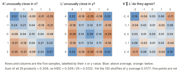
Worked example. The five parabola points, with Gaussian kernels whose bandwidths come from the median heuristic (\sigma = the median distance between two samples): \sigma_x=2, \sigma_y=3. Some cells of Figure 2, read one at a time:
- The diagonal is always positive. \tilde K_{ii} is a squared length (of x_i’s centred feature vector), so it cannot be negative, and neither can \tilde L_{ii}.
- x=-2 against x=-1: neighbours in x (\tilde K=0.24), but y=4 against y=1 is far (\tilde L=-0.18). They disagree: -0.04.
- x=-2 against x=2: as far apart as possible in x (\tilde K=-0.35), identical in y (\tilde L=0.32). They disagree: -0.11. The fold of the parabola maps mirror points to the same y.
- x=-2 against x=1: far apart in both (-0.31 and -0.18). They agree: +0.06.
The 25 products sum to 0.309, so \mathrm{HSIC}_b=0.309/25=0.0123. Is that big? There is only one fair comparison: the same data with the pairing destroyed. Shuffling the five y values gives 120 possible orderings. They average 0.0177, more than the real pairing, and 68 of the 120 score at least 0.0123. Four of those 68 are the real pairing itself: swapping the two 4s or the two 1s changes nothing. So five points carry no evidence of dependence here. The mirror-point disagreements cancel the neighbour agreements.
This is not a bad choice of bandwidth: across a grid of \sigma_x from 0.5 to 3 and \sigma_y from 0.5 to 4.5, the best case still has 44 of the 120 orderings scoring at least as high as the truth. Five points are simply too few. With 200 noisy points (Figure 1) the same parabola gives p=0.001. Two lessons carry forward. A raw HSIC value means nothing until it is compared with shuffles (§7). And \mathrm{HSIC}_b is never negative: it is the trace of a product of two PSD matrices. Even independent data score above zero, partly because the diagonal gives every sum a positive head start.
5. What HSIC measures in the population
The formula above is computed from a sample. The quantity it estimates is a property of the data-generating process. Here \mathbb E[\cdot] means “the average over many random draws”. Draw two pairs (x,y) and (x',y') independently from the joint distribution. Then
\begin{aligned} \mathrm{HSIC} &=\underbrace{\mathbb E\big[k(x,x')\,l(y,y')\big]}_{\text{two genuine pairs}} +\underbrace{\mathbb E\big[k(x,x')\big]\,\mathbb E\big[l(y,y')\big]}_{x\text{'s and }y\text{'s from unrelated draws}}\\[4pt] &\quad-2\,\underbrace{\mathbb E_{x,y}\Big[\mathbb E_{x'}\big[k(x,x')\big]\,\mathbb E_{y'}\big[l(y,y')\big]\Big]}_{\text{one genuine pair against unrelated partners}} . \end{aligned}
Read it as a comparison. The first term measures how much “alike in x” and “alike in y” go together for real pairs. The second is the same measurement when the x values and the y values have nothing to do with each other. The third is the cross term. If x and y are independent, the averages factor and all three terms equal \mathbb E[k]\,\mathbb E[l], so \mathrm{HSIC}=(1+1-2)\,\mathbb E[k]\,\mathbb E[l]=0. The sample version of this expansion, with the three averages taken over the data, equals the trace formula exactly.
HSIC is a distance between two data sets. Build a fake “independent” version of the data by pairing every x_a with every y_b: n^2 pairs, in which any link between x and y is gone by construction. HSIC is the squared MMD (maximum mean discrepancy) between the real cloud of n pairs and this fake cloud, using the similarity k(x,x')\,l(y,y') between pairs.
MMD in one line: map every point to its feature vector, average the feature vectors of each data set, and measure the distance between the two averages. With a characteristic kernel, such as the Gaussian, two different distributions always have different average feature vectors, much as a distribution is pinned down by all its moments. So, in the population,
\mathrm{HSIC}=0\iff p(x,y)=p(x)\,p(y)\iff x\text{ and }y\text{ are independent}.
Gretton et al. (2005) proved this for universal kernels on compact domains, and later work extended it to characteristic kernels, which include the Gaussian kernel on \mathbb R^d. With the linear kernel only the forward direction survives: independence gives HSIC =0, but HSIC =0 only means “no correlation”.
6. Which kernel, and what it can see
| Kernel k(x,x') | Its features | HSIC =0 means |
|---|---|---|
| linear, x\cdot x' | the coordinates themselves | no correlation between any coordinate of x and any of y |
| polynomial, (1+x\cdot x')^d | all monomials up to degree d | no correlation between any such monomials of x and of y |
| Gaussian, e^{-\lVert x-x'\rVert^2/2\sigma^2} | all degrees (§3) | independence |
The Gaussian kernel’s bandwidth \sigma decides what it can actually see from a finite sample. Both extremes throw the advantage away (compare Gram matrix §7):
- Huge \sigma: HSIC becomes linear. For large \sigma, k\approx1-\lVert x-x'\rVert^2/2\sigma^2, and \lVert x_i-x_j\rVert^2=\lVert x_i\rVert^2+\lVert x_j\rVert^2-2x_i\cdot x_j. Centring removes anything that depends on i alone or on j alone (the constant and the two squared lengths), leaving \tilde K\approx\tilde X\tilde X^\top/\sigma^2, the linear kernel. So \mathrm{HSIC}\cdot\sigma_x^2\sigma_y^2\to linear HSIC.
- Tiny \sigma: every shuffle scores the same. When no two samples are within \sigma of each other, K\to I: every point is similar only to itself. Then \tilde K\to H and HSIC \to\frac{1}{n^2}\operatorname{tr}(\tilde L), a number that does not depend on how the y’s are paired with the x’s. A test built on it cannot tell the real pairing from a shuffled one.
Between the two failure modes the parabola is found easily. The median heuristic is the usual default because it puts \sigma at the typical scale of the data, between the two failure modes. It has no optimality guarantee, though. Put points on the dark squares of a 5\times5 checkerboard: the squares are narrower than the typical distance between points, and Pearson r is near zero. At the median bandwidth the test finds nothing. At a fifth of it, the pattern stands out clearly. A kernel wider than the pattern blurs it away. Widget 4 of the interactive page plots this whole curve for any data set.
7. Is it big enough? The permutation test
HSIC is never exactly zero on a sample, so “is it zero?” has to become “is it larger than chance?”. Shuffling answers that. Randomly reorder the y values, keeping the x values where they are. The shuffled data have exactly the same x values and exactly the same y values as before (both marginals are untouched), but any link between them is destroyed. This simulates the independent world with your own data. Repeat 999 times, recompute HSIC each time, and report
p=\frac{1+\#\{\text{shuffles scoring}\ge\text{observed}\}}{1+999}.
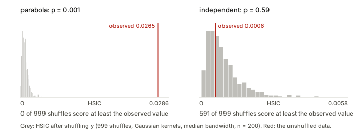
Implementation is cheap. Shuffling y reorders the rows and the columns of L together, and centring commutes with reordering, so \tilde L can be shuffled directly. Each shuffle then costs one n\times n elementwise product.
Why not compare with zero? Because \mathrm{HSIC}_b is positive even under independence. For independent data, the average over shuffles is positive. It shrinks like 1/n but never reaches zero. Song et al. (2012) give an unbiased estimator that removes the diagonal’s head start. Gretton et al. (2007) avoid shuffling altogether by fitting a gamma distribution to the null. For moderate n the shuffle test is the easiest to trust.
8. Normalising: CKA
HSIC’s size depends on the kernels’ scales and on n, so an HSIC of 0.02 means different things in different settings. Normalise it the way correlation normalises covariance:
\mathrm{CKA}(K,L)=\frac{\mathrm{HSIC}(K,L)}{\sqrt{\mathrm{HSIC}(K,K)\,\mathrm{HSIC}(L,L)}} =\frac{\langle\tilde K,\tilde L\rangle_F}{\lVert\tilde K\rVert_F\,\lVert\tilde L\rVert_F}.
This is the cosine of the angle between the two centred Gram matrices, each unrolled into one long vector of n^2 numbers. It lies between 0 and 1, and equals 1 when the two tables are proportional. The name is short for centred kernel alignment.
Kornblith et al. (2019) use it to compare representations. Feed the same n inputs through two layers (or two networks), getting X (n\times p) and Y (n\times q). With linear kernels,
\mathrm{CKA}_{\text{lin}}=\frac{\lVert\tilde X^\top\tilde Y\rVert_F^2}{\lVert\tilde X^\top\tilde X\rVert_F\,\lVert\tilde Y^\top\tilde Y\rVert_F},
the feature-side form of §2, which stores a p\times q matrix instead of two n\times n ones. Linear CKA is the same quantity as the older RV coefficient of multivariate statistics. Linear CKA ignores rotations and overall scale, as a comparison of embedding spaces should (Gram matrix §3). It is not invariant to every invertible linear map, unlike CCA. Kornblith et al. argue that this is deliberate: a similarity index that ignores all invertible linear maps gives the same answer for any two representations whose rank equals the number of examples, which is the usual situation once a layer is wider than the data set. Such an index cannot tell them apart.
High-variance directions dominate. Diagonalise both centred Gram matrices, \tilde K=\sum_i\lambda_iu_iu_i^\top and \tilde L=\sum_j\mu_jv_jv_j^\top. Then
\langle\tilde K,\tilde L\rangle_F=\sum_{i,j}\lambda_i\,\mu_j\,(u_i\cdot v_j)^2 ,
so each pair of principal directions counts in proportion to the product of their variances. Take two representations that share exactly one direction and are otherwise unrelated noise. If the shared direction has the same variance as the others, linear CKA is small. Make that one direction much higher in variance and linear CKA becomes large, even though nine of ten directions are still unrelated.
9. Relatives: COCO, HGR maximal correlation and the H-score
HSIC sums the squared singular values of the cross-covariance operator, \mathrm{HSIC}=\sum_k s_k^2. Its relatives summarise the same kind of object differently:
| Measure | What it keeps | Normalised? |
|---|---|---|
| HSIC | \sum_k s_k^2, all directions | no: covariances |
| COCO, constrained covariance (Gretton et al., JMLR 2005) | s_1, the single best pair of features f,g | no |
| kernel canonical correlation (Bach & Jordan, JMLR 2002) | the best pair, divided by their spreads (with regularisation) | yes: correlations |
| HGR maximal correlation (inequalities page) | the best pair over all functions | yes |
| \chi^2(P_{XY}\Vert P_XP_Y) and the H-score (Bao et al. note) | \lVert\tilde B\rVert_F^2, a sum of squared maximal correlations | yes |
In the random linear example of §2 the top singular value is s_1=1.0623, so s_1^2=1.1284 out of HSIC’s 1.1545: 97.7% of the dependence lies along one direction, and HSIC also counts the rest. The last row is worth dwelling on, because it has the same shape as HSIC: build a matrix that is zero exactly under independence, then sum its squared singular values. The H-score note’s \tilde B does it with probabilities normalised by the marginals, and HSIC does it with kernel covariances. Kernel canonical correlation approaches HGR as the kernel becomes rich and the regularisation vanishes.
10. Where it shows up
- Independence tests (Gretton et al., NeurIPS 2007): the construction of §7.
- Feature selection (Song, Smola, Gretton, Bedo & Borgwardt, JMLR 2012): keep the features whose HSIC with the labels is largest. This paper also gives the unbiased estimator.
- Comparing networks: CKA (Kornblith et al., ICML 2019), §8.
- Removing an unwanted dependence: add HSIC as a penalty. ReBias (Bahng et al., ICML 2020) makes a model’s features independent of those of a deliberately biased model. Greenfeld & Shalit (ICML 2020) make a regression’s residuals independent of its inputs, for robustness to covariate shift.
- Self-supervised learning: SSL-HSIC (Li, Pogodin, Sutherland & Gretton, NeurIPS 2021) maximises HSIC between representations and image identity, and shows that InfoNCE implicitly approximates a version of it (compare the InfoNCE note).
- Training without backpropagation: the HSIC bottleneck (Ma, Lewis & Kleijn, AAAI 2020) trains each layer to maximise HSIC with the labels while minimising it with the inputs.
- Domain alignment in the MICCAI 2026 DA notes uses MMD between source and target features. HSIC is the same tool pointed at a different pair: the joint distribution against the product of its marginals (§5).
Questions and doubts
- The bandwidth decides what HSIC can see (§6), yet the default is a heuristic with no optimality property. Choosing \sigma to maximise the test statistic on the same data you then test invalidates the p-value, unless the data are split first.
- How many samples does a given dependence need? Five points could not show a noise-free parabola at any bandwidth tried, while 200 noisy ones showed it at p=0.001. The power depends on n, the kernel and the shape of the dependence together, and there is no simple rule. The n slider in widget 1 gives a feel for it.
- CKA’s eigen-weighting (0.125 against 0.888 for one shared direction) means a claim that “these two layers are similar” may rest on a handful of high-variance directions. Reporting CKA after whitening, or alongside a per-direction breakdown, would make such claims easier to trust.
- HSIC is symmetric. It says that x and y are related, not which drives which, and it counts all dependence equally, whether or not it is the useful kind.
- The Gram matrices are n\times n: 10^4 samples means 10^8 entries each. Random Fourier features and Nyström approximations make this cheaper. How much they change the calibration of the permutation test is worth checking before relying on them.
- When HSIC is a training penalty (ReBias, Greenfeld & Shalit), it is estimated on mini-batches. The null mean alone shrinks only like 1/n, so at a small batch size it may be comparable to the dependence being removed. Whether the penalty then targets real dependence or estimator noise seems under-examined.
Takeaways
- \mathrm{HSIC}_b=\frac{1}{n^2}\sum_{ij}\tilde K_{ij}\tilde L_{ij}: do the two centred Gram matrices agree about which pairs of samples are alike?
- With a linear kernel it is the squared covariance, or \lVert C\rVert_F^2 for vectors, and it is blind to parabolas, circles and funnels. With a Gaussian kernel it has features of every degree and is zero only under independence.
- “Hilbert–Schmidt” is the Frobenius norm of the covariance table between all features of x and all features of y.
- HSIC is the MMD between the joint distribution and the product of its marginals.
- Judge it against shuffles, never against zero. Too wide a bandwidth makes it linear, and too narrow a bandwidth makes it blind.
- CKA is the cosine between two centred Gram matrices. It ignores rotation and scale, and it is dominated by high-variance directions.