Understanding Contrastive Representation Learning through Alignment and Uniformity on the Hypersphere
Links
- arXiv:2005.10242 — use this version, not the ICML proceedings PDF. The arXiv copy carries the supplement and a changelog correcting Theorem 1’s convergence rate (see below).
- Runnable
code — all four claims below checked numerically.
make verifyruns it. - Downstream in this repo: Betser et al. 2026 (whose \Phi(\mu) is Theorem 1’s second term) and Zhang et al. 2026 (which inherits this decomposition).
In one paragraph
Everyone “knew” contrastive learning pulls positives together and pushes negatives apart. This paper makes that precise and, more importantly, shows the two halves are separable, nameable, and individually measurable. Taking M \to \infty negatives, the InfoNCE loss splits exactly into an alignment term (minimised iff positive pairs map to identical features) and a uniformity term (minimised iff the feature distribution is uniform on the sphere). The uniformity term turns out to be an energy from classical potential theory, which is why the uniform measure is its unique minimiser. The paper then proposes \mathcal{L}_{align} and \mathcal{L}_{uniform} as standalone losses and shows that optimising them directly matches or beats the contrastive loss — the strongest possible evidence that the decomposition captures what the loss was doing.
The spine of the argument
- Drop the InfoMax framing. The MI-bound story is empirically falsified, so analyse what the loss actually optimises instead of what it bounds.
- Take M\to\infty and normalise by \log M. The loss splits cleanly in two (Theorem 1).
- The first term is minimised exactly at perfect alignment. Immediate.
- The second term is an average pairwise Gaussian potential, so classical potential theory applies: strict positive definiteness gives a unique minimiser, and rotational symmetry forces it to be uniform (Propositions 1 and 2).
- That same term is a resubstitution entropy estimator, so minimising it is maximising the estimated entropy of the features.
- Turn both halves into standalone metrics and show they predict downstream accuracy and work as training objectives.
Setup and notation
| Symbol | Meaning |
|---|---|
| p_{data}, p_{pos} | data distribution; distribution of positive pairs |
| f : \mathbb{R}^n \to S^{m-1} | encoder onto the unit sphere |
| \tau, M | temperature; number of negatives |
| \sigma_d | normalised surface measure on S^d — “the uniform distribution” |
| G_t(u,v) | Gaussian / RBF potential e^{-t\lVert u-v\rVert^2} |
| I_K[\mu] | energy \iint K(u,v)\,d\mu\,d\mu |
| t, \alpha | RBF bandwidth (t=2) and alignment exponent (\alpha=2) |
| \hat H, \hat I | resubstitution entropy estimator; the MI estimator built from it |
| \kappa = 1/\tau | vMF concentration, when the second term is read as a KDE |
The two assumptions, and which one matters
Symmetry p_{pos}(x,y)=p_{pos}(y,x) does light work: it lets you stop distinguishing anchor from positive.
Matching marginal \int p_{pos}(x,y)\,dy = p_{data}(x) is load-bearing, in two ways.
It collapses two distributions into one. In Theorem 1’s limit the second term is \mathbb{E}_{(x,y)\sim p_{pos}} \log \mathbb{E}_{x^-\sim p_{data}}[e^{f(x^-)^\top f(x)/\tau}]. The inner expression depends only on the anchor, so the outer expectation reduces to one over the marginal of p_{pos}. Matching marginal says that marginal is p_{data} — the same law the negatives come from. Without it you have anchors from one distribution and negatives from another, the second term stops being a functional of a single feature distribution, and the whole “uniformity of the feature distribution” reading collapses.
It makes uniformity well-defined. Perfect uniformity is a statement about the law of f(x) for x\sim p_{data}. Matching marginal is what makes “spread the negatives out” and “the feature distribution is uniform” the same sentence.
It holds by construction when positives are two i.i.d. augmentations of one base sample — but it fails for MoCo-style memory banks, whose features come from an older momentum encoder and so are not distributed as f_\#p_{data} for the current f. The analysis assumes this away.
InfoMax is not what InfoNCE does
InfoMax is a principle (maximise I(f(x);f(y))); InfoNCE is a loss. The bridge is that -\mathcal{L}_{contrastive} + \log M lower-bounds the mutual information. Wang & Isola’s position is that the bridge is broken, citing Tschannen et al. (2019): optimising a tighter MI bound often yields worse representations. If the MI story explained the success, tighter would be better.
Two structural reasons it cannot be right:
- MI is invariant to invertible transformations of f, so it cannot distinguish a linearly separable representation from an information-equivalent scrambled one — precisely the property a linear probe measures.
- The bound saturates at \log M, yet performance keeps improving with M well past where the bound could be tracking anything.
Their reconciliation via I(f(x);f(y)) = H(f(x)) - H(f(x)\mid f(y)) is the useful part: uniformity does correspond to maximising H(f(x)), but alignment is strictly stronger than minimising H(f(x)\mid f(y)) — it demands f(x)=f(y) a.s., where low conditional entropy only demands predictability. So the loss optimises something adjacent to MI: aligned and information-preserving.
Why a Gaussian potential, and not something simpler
The requirement is a functional on distributions over S^d that is uniquely minimised by uniform, sensible with finitely many points, and cheap.
The obvious candidates fail badly. \mathbb{E}[u^\top v] = \lVert\mathbb{E}[u]\rVert^2, so average dot product is minimised by any zero-mean distribution; average squared distance is the same thing in disguise, since \lVert u-v\rVert^2 = 2-2u^\top v on the sphere.
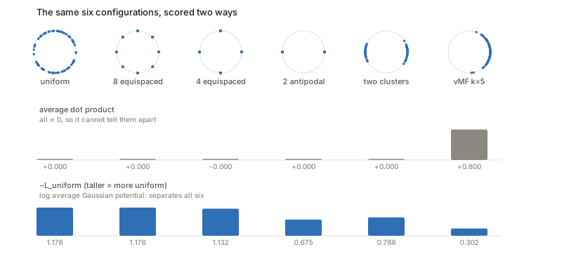
What you need is a kernel whose energy is strictly positive definite: I_K[\mu] \ge 0 for every signed measure with equality only at \mu\equiv 0. That makes the energy strictly convex over measures, which buys a unique minimiser.
Among strictly PD kernels the Gaussian is chosen because it is bounded and singularity-free, it is tied to universally optimal configurations (Cohn & Kumar), it can represent a general class of other kernels including the Riesz s-potentials — and, decisively for this paper, on the sphere it is exponentiated cosine similarity:
G_t(u,v) = e^{-t\lVert u-v\rVert^2} = e^{2t\,u^\top v - 2t}
The object inside the InfoNCE softmax is a Gaussian
potential. Without that identity there is no Theorem 1. (Checked to
10^{-16} in code/.)
Unpacking \mathcal{L}_{uniform}
\mathcal{L}_{uniform}(f;t) = \log \mathbb{E}_{x,y \overset{iid}{\sim} p_{data}}\big[e^{-t\lVert f(x)-f(y)\rVert^2}\big]
Three layers, inside out. G_t is a crowding measure for a pair, near 1 when the points coincide and near 0 when they are far apart. The expectation is the total energy of the configuration — think of each feature as a charge repelling every other. The \log is monotone and therefore changes nothing about the minimiser; it is there for numerical scale, to match the log-scale of the contrastive loss, and for gradient conditioning.
Range: \mathbb{E}[G_t]\in(0,1], so \mathcal{L}_{uniform}\le 0, hitting 0 in the worst case where all points collapse.
Proposition 1, unpacked
Claim: \sigma_d is the unique minimiser of I_{G_t}[\mu] over Borel probability measures on S^d.
The paper’s proof is one line — “a direct consequence of Lemmas 1 and 2” — with both lemmas imported from Borodachov, Hardin & Saff (2019): G_t is strictly PD on S^d, and for a strictly PD kernel of the form f(\lVert u-v\rVert^2) with finite energy, \sigma_d is the unique minimiser and finite-point minimisers converge weak* to it.
Why strict positive definiteness gives uniqueness. Suppose \mu_1,\mu_2 both minimise. Put \nu = \mu_1-\mu_2, a signed measure with \nu(S^d)=0. Then
I[\mu_1] = I[\mu_2+\nu] = I[\mu_2] + 2\!\iint\! G_t\,d\mu_2\,d\nu + I[\nu].
At a minimum the cross term vanishes, and strict PD forces I[\nu]>0 unless \nu\equiv 0. It is the measure-space analogue of “a strictly convex function has one minimum.”
Why that minimiser is \sigma_d — a symmetry argument the paper leaves implicit. G_t depends only on \lVert u-v\rVert, so the energy is rotation-invariant. If \mu^* is the unique minimiser then R_\#\mu^* = \mu^* for every rotation R, and the only rotation-invariant probability measure on the sphere is \sigma_d.
Strict PD gives uniqueness; symmetry then identifies it for free. Proposition 2 is the finite-N half of the same lemma, which is why 8 equispaced points score marginally better than a sampled uniform in the figure above — no contradiction, just Proposition 2 in action.
Theorem 1, and a correction
\lim_{M\to\infty}\big[\mathcal{L}_{contrastive}(f;\tau,M) - \log M\big] = -\tfrac{1}{\tau}\mathbb{E}_{p_{pos}}[f(x)^\top f(y)] + \mathbb{E}_{x\sim p_{data}}\log\mathbb{E}_{x^-\sim p_{data}}\big[e^{f(x^-)^\top f(x)/\tau}\big]
The derivation is short. Split the log of the fraction, subtract \log M and push it inside:
\mathcal{L} - \log M = -\tfrac{1}{\tau}\mathbb{E}[u^\top v] + \mathbb{E}\Big[\log\Big(\tfrac{1}{M}e^{u^\top v/\tau} + \tfrac{1}{M}\textstyle\sum_i e^{u_i^-{}^\top v/\tau}\Big)\Big]
As M\to\infty the first inner term is one bounded quantity over M and vanishes; the second is an average of i.i.d. bounded terms, so the SLLN sends it to \mathbb{E}_{x^-}[e^{f(x^-)^\top f(y)/\tau}]. The Continuous Mapping Theorem pushes the limit through the \log, bounded convergence swaps limit and expectation (everything lives in [e^{-1/\tau}, e^{1/\tau}]), and matching marginal converts the outer expectation.
Why \log M must be subtracted: without it the loss diverges, since the sum has M terms. It is the entropy of a uniform choice among the candidates. Practical corollary: raw InfoNCE values are not comparable across batch sizes.
Result 1 is immediate — on the sphere u\cdot v = 1 - \lVert u-v\rVert^2/2, so minimising -\mathbb{E}[u\cdot v] is minimising \mathbb{E}\lVert f(x)-f(y)\rVert^2, zero iff perfectly aligned.
The rate: two corrections, one of them mine
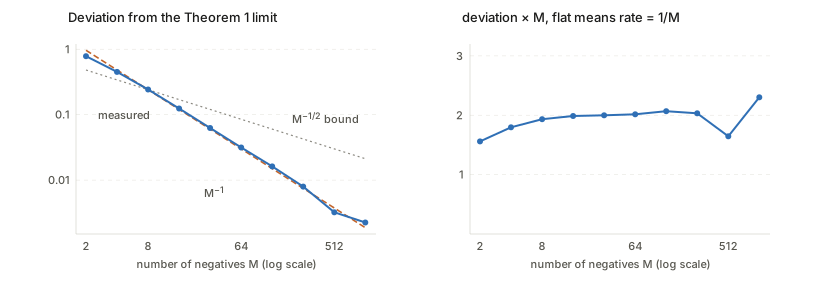
- The published rate is superseded. The ICML proceedings version states O(M^{-2/3}). The arXiv changelog dated 11/6/2020 reads “Corrected Theorem 1’s convergence rate to O(M^{-1/2}).” If you cite the rate, cite M^{-1/2} and use the arXiv version.
- Even the corrected rate is loose, by a factor of \sqrt M. Their proof bounds \mathbb{E}\lvert\log A_M - \log \mathbb{E}A\rvert \le c\,\mathbb{E}\lvert A_M - \mathbb{E}A\rvert = O(M^{-1/2}) via the mean value theorem plus Berry–Esseen — taking absolute values before the expectation, which discards the cancellation of the mean-zero first-order term. A delta-method expansion keeps it: \mathbb{E}[\log A_M] - \log\mathbb{E}[A] \approx -\operatorname{Var}(A_M)/(2(\mathbb{E}A)^2) = O(1/M). Their bound is valid, just not tight; the measurement above agrees with the delta method.
The resubstitution entropy estimator
With p_{data} uniform over a finite dataset the second term becomes a double sum, \frac{1}{N}\sum_i \log\big[\frac{1}{N}\sum_j e^{f(x_i)^\top f(x_j)/\tau}\big]. Now recognise the inner sum: the von Mises–Fisher density is p_{vMF}(u;\mu,\kappa) = Z_{vMF}^{-1}e^{\kappa\mu^\top u}, so with \kappa = 1/\tau each term is Z_{vMF}\cdot p_{vMF}(f(x_i); f(x_j), 1/\tau) and the average is a kernel density estimate of the feature distribution evaluated at f(x_i), built from the features themselves as kernel centres with bandwidth \tau. Hence
\text{second term} = \underbrace{\tfrac{1}{N}\textstyle\sum_i \log \hat p_{\text{KDE}}(f(x_i))}_{=\,-\hat H(f(x))} + \log Z_{vMF}.
“Resubstitution” names the trick: estimate H = -\mathbb{E}[\log p(X)] by fitting \hat p on the sample and evaluating it at that same sample. So minimising the second term is maximising the estimated entropy of the features, and uniform is the max-entropy law on the sphere — which is Result 2.
Two caveats worth carrying. The estimator is biased: the j=i term contributes e^{1/\tau}, the largest value possible, so every point inflates its own density. That bias is configuration-independent, so the argmin is unaffected, but the value is not a good entropy estimate. And since f is deterministic, \hat H(f(x)) doubles as an estimator of \hat I(x; f(x)) — the source of “information-preserving”.
The two metrics, and what the logsumexp is doing
\mathcal{L}_{align}(f;\alpha) = \mathbb{E}_{p_{pos}}\big[\lVert f(x)-f(y)\rVert_2^\alpha\big], \qquad \mathcal{L}_{uniform}(f;t) = \log \mathbb{E}_{x,y}\big[e^{-t\lVert f(x)-f(y)\rVert_2^2}\big]
The chain from “logsumexp of an RBF” to “uniformity” has four links: the RBF on the sphere is exponentiated cosine similarity; averaging it gives an energy; strict positive definiteness makes uniform the unique minimiser; and the placement of the \log distinguishes the two forms.
- \mathcal{L}_{uniform} = \log\mathbb{E}_x\mathbb{E}_y[G_t] — log outside both.
- Theorem 1’s second term = \mathbb{E}_x\log\mathbb{E}_y[G_t] + 1/\tau — log between them. Over a finite batch, \log\mathbb{E}_y is a logsumexp minus \log M.
By Jensen, \mathbb{E}_x\log\mathbb{E}_y[G] \le \log\mathbb{E}_x\mathbb{E}_y[G], with equality iff \mathbb{E}_y[G(x,\cdot)] is constant in x — which is exactly the uniformity equilibrium condition: every point feels the same total potential from the rest.
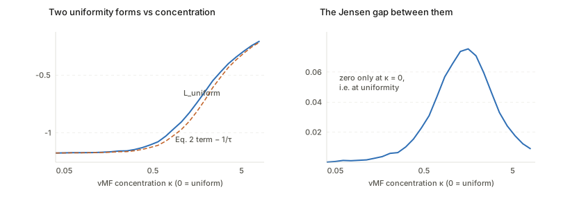
Why prefer \mathcal{L}_{uniform} in practice: one scalar over all pairs, a single logsumexp over the batch’s pairwise distances, instead of a per-anchor softmax with its expensive normalisation. And a final intuition — logsumexp is a soft maximum, so as t\to\infty the metric is dominated by the single closest pair and degenerates into the best-packing (Tammes) objective. At finite t it weights all pairs but emphasises the crowded ones, which is why it behaves sensibly with finitely many points rather than only in the limit.
Questions and doubts
- Perfect alignment and perfect uniformity are jointly unachievable on finite data, as the paper itself notes: perfect alignment forces every augmentation of one sample to a single point, which cannot be uniform. So the two metrics are always in tension and the “optimum” is a trade-off the theory does not characterise. The experiments tune the weighting by hand.
- Matching marginal excludes the memory-bank methods the paper repeatedly cites as motivation (MoCo). Not acknowledged.
- t and \alpha are free parameters with no theory guiding them. Proposition 1 holds for every t>0, so the asymptotic claim gives no way to choose one; the paper picks t=2, \alpha=2 empirically.
- The entropy-estimator reading is suggestive rather than tight. The estimator is biased by a self-term, and KDE entropy estimation on a sphere in m dimensions with N points is a poor estimator for realistic m. The identification is exact as algebra, loose as statistics.
- The rate in the published version is wrong and even the corrected one is loose — see above. Worth knowing before citing it.
Takeaways
- The decomposition is the contribution, and it is unusually clean: one loss, two terms, each with an exact characterisation of its minimiser.
- The uniformity term is an energy from potential theory, and recognising that is what turns a vague “spread out” intuition into a theorem with a unique minimiser.
- Strict positive definiteness is the property to remember. It is what separates a usable uniformity objective from a degenerate one, and why the RBF works where the dot product cannot.
- Minimising the repulsion term is maximising an entropy estimate of the feature distribution — a cleaner statement of “information-preserving” than the MI-bound framing it replaces.
- That optimising \mathcal{L}_{align} + \mathcal{L}_{uniform} directly matches the contrastive loss is the strongest evidence for the analysis: the decomposition is not just descriptive, it is sufficient.