The Price of Robustness: Stable Classifiers Need Overparameterization
Links
- OpenReview: the ICLR 2026 page. arXiv:2603.02806: the preprint. No code is released.
- Interactive
companion: five widgets. (1) Margin, class stability and
co-stability for 2-D classifiers you can bend, including a 1-NN
memoriser. (2) Isoperimetry: histograms of Lipschitz functions of a
Gaussian as the dimension grows. (3) The surrogate trick that every
proof uses, as a trade-off you can slide, plus the paper’s Example 9.
(4) The law of robustness as a calculator.
- The toy experiment below, rerun in the browser.
- Runnable
checks:
stability_checks.pychecks the Lipschitz facts, the union-bound algebra, the tail-to-mean step, the contraction in Eq 2, the scales, and Corollary 15 as stated.rf_margin_toy.pyis the toy law of robustness. Every number below comes from one of them.make verifyruns both. - Inequalities and concentration: the Rademacher complexity and concentration on the sphere sections are the background this paper assumes.
- The four fundamental subspaces: the minimum-norm interpolant used in the toy experiment, and why it is the one gradient descent from zero finds.
- The paper it extends: Bubeck and Sellke, A universal law of robustness via isoperimetry, NeurIPS 2021 (arXiv:2105.12806).
Jonas von Berg, Adalbert Fono, Massimiliano Datres, Sohir Maskey and Gitta Kutyniok, The Price of Robustness: Stable Classifiers Need Overparameterization, ICLR 2026. LMU Munich and the Munich Center for Machine Learning.
In one paragraph
Bubeck and Sellke (2021) proved a law of robustness for regression. If a model with p parameters fits n noisy points in d dimensions, its Lipschitz constant must be at least about \sqrt{nd/p}. So a smooth fit needs p\approx nd parameters, far more than the p\approx n needed just to fit. That result is useless for classifiers, because a classifier f=\operatorname{sgn}\circ g jumps and has no finite Lipschitz constant. Rescaling g also changes g’s Lipschitz constant without changing f at all. This paper swaps the Lipschitz constant for a geometric quantity that belongs to f alone: the class stability S(f)=\mathbb E[h_f(x)], the average distance from a data point to the decision boundary. Its main result (Theorem 4) bounds the Rademacher complexity of a finite class of classifiers by roughly \frac{1}{S}\sqrt{c\log|\mathcal F|/(nd)}, where c measures how concentrated the data are. The corollary (Corollary 6) is the classification law of robustness: any classifier that fits the training set below the noise level has S(f)\lesssim \frac{1}{\varepsilon}\sqrt{cp/(nd)}. A memoriser with p\approx n parameters therefore has margins no larger than the \sqrt{c/d} that a random hyperplane gets for free. To have margins of order one it needs p\gtrsim nd. Section 5 extends this to infinite, parameterised classes by adding a second, output-space margin (the normalized co-stability \mathbb E|g|/L(g)). The experiments show stability growing with width on MNIST and CIFAR-10. The mathematics is mostly sound, and the central trick is neat. I found one statement that is wrong as written (Corollary 15 drops a term, and without it the law loses its dependence on p). One proof is weaker than it needs to be: Theorem 4.1 is vacuous in the regime it is meant for, and Theorem 4.2’s extra assumptions can be dropped. The experiments never reach the regime the theorem is about.
Background, from the ground up
Why the Lipschitz constant is the wrong ruler for a classifier
A function is L-Lipschitz if moving the input by r moves the output by at most Lr. For regression that is the natural notion of robustness: a small L means a small perturbation cannot change the prediction much. A classifier outputs only \pm1, so any classifier that is not constant jumps by 2 somewhere and has L=\infty. The usual fix is to look at the score g inside f=\operatorname{sgn}\circ g. But g and 10g give the same classifier, and their Lipschitz constants differ by a factor of 10. So “the Lipschitz constant of the score” measures the representation, not the classifier.
What does belong to the classifier is the geometry of its decision boundary: how far a typical input is from the nearest input that f labels differently. That distance is the margin in the input space, and its average is what the paper calls class stability. Widget 1 of the interactive page lets you rescale g and watch the margin stay put.
Generalisation, and Rademacher complexity as “how well can this class fit noise?”
A classifier generalises when its error on fresh data (the risk R(f)) is close to its error on the training set (the empirical risk \hat R(f)). The classical uniform bound says that, with probability at least 1-\delta, for every f in the class at once,
R(f)-\hat R(f) \;\le\; 2\,\mathcal R_{n,\mu}(\ell\circ\mathcal F) + a\sqrt{\frac{2\log(2/\delta)}{n}} \qquad\text{(Eq 1)}
where a bounds the loss. The key quantity is the Rademacher complexity. The idea first: flip n fair coins \sigma_i\in\{-1,+1\} to get a completely random labelling of the n training points. Then ask how well the best function in the class can line up with that noise. A class that can match any random labelling can memorise, and its training error says nothing about its test error. A class that cannot is forced to learn structure. In symbols,
\mathcal R_{n,\mu}(\mathcal F) = \frac1n\,\mathbb E_{\sigma,x}\Big[\sup_{f\in\mathcal F}\Big|\sum_{i=1}^n \sigma_i f(x_i)\Big|\Big].
Here \sum_i\sigma_i f(x_i) counts agreements minus disagreements between f and the coin flips, and the sup picks the best-matching f. Two small examples with n=4:
- If \mathcal F contains all 16 labellings of the four points, some f always matches the coins exactly. The sum is 4, and \mathcal R=1: the class fits pure noise.
- If \mathcal F=\{+1,-1\} (the two constant classifiers), the best you can do is |\sum_i\sigma_i|. Over the 16 coin patterns this takes the values 4, 2, 0, 2, 4 with counts 1, 4, 6, 4, 1. The mean is 24/16=1.5, so \mathcal R=1.5/4=0.375.
For a finite class, Massart’s lemma gives \mathcal R\lesssim\sqrt{\log|\mathcal F|/n}, whatever the data. The paper wants something better: a bound that shrinks when the classifiers are stable. For the 0–1 loss \ell_{0\text{-}1}(f(x),y)=\mathbb 1[f(x)\ne y]=(1-yf(x))/2, the complexity of the loss class is half that of \mathcal F (Eq 2). So it suffices to bound \mathcal R_{n,\mu}(\mathcal F).
Isoperimetry: in high dimension, Lipschitz functions are nearly constant
The paper’s only assumption on the data is isoperimetry. The idea first: draw x from a high-dimensional Gaussian scaled so that \lVert x\rVert\approx1, say x\sim\mathcal N(0,I_d/d). Its first coordinate x_1 has standard deviation 1/\sqrt d. Its length \lVert x\rVert is also within about 1/\sqrt{2d} of 1. The same holds for the distance from x to any fixed set of points. Every 1-Lipschitz function of x fluctuates by only O(1/\sqrt d) around its mean. That is concentration of measure: in high dimension the mass of a nice distribution sits in a thin shell, and a function that cannot change quickly cannot tell the points of the shell apart.
Formally (Definition 3), \mu is c-isoperimetric if for every bounded L-Lipschitz f and every t\ge0,
\mathbb P\big(|f(x)-\mathbb E f|\ge t\big) \;\le\; 2\exp\!\Big(-\frac{d\,t^2}{2cL^2}\Big). \qquad\text{(Eq 3)}
Reading the symbols: d is the
dimension, L the Lipschitz constant,
and c a constant that absorbs the scale
of the data. For \mathcal N(0,I_d/d),
c=1. The typical fluctuation is L\sqrt{c/d}. Uniform measures on spheres and
positively curved manifolds also qualify, with d the intrinsic dimension. Widget 2 of the interactive page shows the
histograms narrowing. stability_checks.py §7 measures
standard deviations of 0.224, 0.157 and 0.149 for x_1, \lVert
x\rVert and the distance to 5 fixed points at d=20, and 0.071, 0.050 and 0.051 at d=200.
Compare Hoeffding’s inequality, which knows only that f\in[-1,1] and gives 2e^{-t^2/2} with no d. Isoperimetry is sharper exactly when L<\sqrt{d/c} (App A.1). This single comparison explains the shape of every result in the paper. A classifier with margin S behaves, on most of the space, like a function with Lipschitz constant about 2/S. So isoperimetry buys something only when 2/S\lesssim\sqrt{d/c}, that is, when S\gtrsim\sqrt{c/d}.
The regression law it extends, in one paragraph
Bubeck and Sellke consider a finite class of L-Lipschitz regressors with \log|\mathcal F|\approx p and labels with noise. A random labelling is fitted only if the functions can wiggle by order one over the sample. Isoperimetry says an L-Lipschitz function wiggles by only L\sqrt{c/d} on typical points, and a union bound over |\mathcal F|=e^p functions contributes a factor \sqrt{p/n}. Balancing the two gives: fitting below the noise level forces L\gtrsim\sqrt{nd/(cp)}. With p\approx n that is L\gtrsim\sqrt d, very non-smooth. To get L=O(1) you need p\gtrsim nd. This paper runs the same argument with 2/S in the role of L.
The spine of the argument
- Define a margin that belongs to f (Def 1). h_f(x) is the distance from x to the nearest point with the other label, and S(f)=\mathbb E h_f.
- Away from the boundary, a classifier is Lipschitz. On the set where h_f\ge m, f is (2/m)-Lipschitz, because two points with different labels there are at least m apart.
- The margin concentrates (Fact 2). h_f is 1-Lipschitz, so by isoperimetry \mathbb P(h_f<S(f)/2)\le e^{-dS(f)^2/(8c)}. Almost every point sits in the good region.
- Replace f by a Lipschitz surrogate that agrees with it on the good region (a McShane extension, or the ramp \operatorname{sgn}_\gamma\circ d_f). Bubeck and Sellke’s lemma bounds its Rademacher complexity by \frac1S\sqrt{c\log|\mathcal F|/(nd)}.
- Pay for the disagreement. The surrogate differs from f only on the thin bad region, whose mass is exponentially small (step 3). This gives Theorem 4.
- Turn the complexity bound into a law (Corollary 6). If all stable classifiers generalise, none of them can fit below the noise level. So any classifier that does fit below the noise level is unstable: S(f)\lesssim\frac1\varepsilon\sqrt{cp/(nd)}.
- For infinite classes, closeness in parameters must mean closeness of classifiers. That fails for \operatorname{sgn} (Example 9). So the paper adds a margin in the output, |g(x)|, and controls its ratio to L(g) (Def 10, Theorem 13, Corollary 15).
Setup and notation
| Symbol | Meaning |
|---|---|
| \mathcal X\subset\mathbb R^d, \mu | bounded input space; the data distribution on \mathcal X\times\{-1,1\} |
| n, d | number of training points, input dimension |
| \mathcal F | the hypothesis class of classifiers f:\mathcal X\to\{-1,1\}; finite in Sec 4 |
| p=\log\lvert\mathcal F\rvert | the “number of parameters”. A p-parameter model discretised on a grid has \log\lvert\mathcal F\rvert=O(p) |
| d(x,A)=\inf_{y\in A}\lVert x-y\rVert_2 | distance from a point to a set |
| d_f(x) | signed distance to the boundary: +d(x,f^{-1}(-1)) if f(x)=1, -d(x,f^{-1}(1)) if f(x)=-1 |
| h_f(x)=\lvert d_f(x)\rvert | the (input) margin: distance to the nearest point labelled differently |
| S(f)=\mathbb E[h_f] | class stability |
| c | isoperimetry constant (Def 3); \sqrt{c/d} is the natural fluctuation scale |
| \mathcal R_{n,\mu} | Rademacher complexity; \sigma_i are independent fair \pm1 coins |
| R(f), \hat R(f), R^* | population risk, empirical risk, best population risk in the class |
| g, L(g) | a score with f=\operatorname{sgn}\circ g, and its Lipschitz constant in x |
| h^*_g=\lvert g\rvert, S^*(g)=\mathbb E\lvert g\rvert | co-margin, co-stability (margins in the output) |
| \bar S^*(g)=S^*(g)/L(g) | normalized co-stability |
| \operatorname{sgn}_\gamma | the ramp: -1 below -\gamma, t/\gamma on [-\gamma,\gamma], +1 above \gamma |
| \mathcal W, W, J | parameter set, its diameter bound, the Lipschitz constant of w\mapsto g_w in sup-norm |
| K, K_1, K_2, C_i | unspecified absolute constants |
Definition 1 and Remark 2: margins, signed distances, class stability
The margin of f at x is
h_f(x)=\inf\{\lVert x-z\rVert_2:\ z\in\mathcal X,\ f(z)\ne f(x)\},
the radius of the largest ball around x that f labels uniformly. The class stability is its average under the data, S(f)=\mathbb E[h_f(x)]. Three things to notice.
- It is an average, not a minimum. Classical margin bounds use the smallest margin on the sample, or a quantile. One training point sitting on the boundary does not destroy S(f).
- It is measured under the data distribution. A boundary can be jagged in empty regions of space at no cost.
- A worked example. For x\sim\mathcal N(0,I_d/d) and the halfspace f=\operatorname{sgn}(x_1), the margin is |x_1| and S(f)=\sqrt{2/(\pi d)}. That is 0.0564 at d=200 (§7 of the checks measures 0.0565). A hyperplane through the middle of the data therefore gets a margin of order \sqrt{c/d} for free. This is the benchmark to keep in mind when reading the corollaries.
Remark 2 and Lemmas 17–18. The signed distance d_f is 1-Lipschitz if \mathcal X is path-connected. If f^{-1}(1) is closed, then f=\operatorname{sgn}\circ d_f, with \operatorname{sgn}(0)=1. The proof of Lemma 17 has two cases. If f(x)=f(y), both values are distances to the same set, and a distance to a fixed set is 1-Lipschitz. If f(x)=1 and f(y)=-1, walk along the segment from x to y. Let w_1 be the first point labelled -1 and w_2 the last point labelled +1. Path-connectedness puts w_1 no later than w_2 on the segment, so
|d_f(x)-d_f(y)| = d(x,f^{-1}(-1))+d(y,f^{-1}(1)) \le \lVert x-w_1\rVert+\lVert y-w_2\rVert \le \lVert x-y\rVert.
Connectedness matters for the signed distance. On \mathcal X=[0,1]\cup[2,3] with f=+1 on the first piece, d_f(1)=+1 and d_f(2)=-1, so d_f changes by 2 over a distance of 1. On a random finite point cloud the measured Lipschitz constant of d_f is exactly 2 (checks §1). The unsigned margin h_f needs no connectedness at all. If f(x)\ne f(y), then y is a candidate for x’s nearest flip and vice versa. So both h_f(x) and h_f(y) lie in [0,\lVert x-y\rVert], and their difference does too. The measured constant is 1.000 on the same point cloud. This small observation comes back in the doubts section.
Eqs 1–2: from generalisation to the Rademacher complexity of \mathcal F
Everything reduces to bounding \mathcal R_{n,\mu}(\mathcal F). The step from the loss class to \mathcal F is the identity \mathbb 1[f(x)\ne y]=\tfrac12-\tfrac12 yf(x). The constant \tfrac12 contributes \tfrac12\sum_i\sigma_i, which has mean zero. Multiplying \sigma_i by the fixed sign y_i does not change its distribution. So without the absolute value inside the sup, \mathcal R(\ell_{0\text{-}1}\circ\mathcal F)=\tfrac12\mathcal R(\mathcal F) exactly. The paper’s definition has the absolute value. Then the constant term no longer averages out, and the correct statement is \le\tfrac12\mathcal R(\mathcal F)+\tfrac1{2\sqrt n}. Exact enumeration on 6 classifiers and 10 points gives 0.3557 for the left side, against \tfrac12\mathcal R(\mathcal F)=0.2537 (checks §8). The extra 1/(2\sqrt n) is absorbed by the 1/\sqrt n already in every bound, so nothing downstream changes.
Theorem 4: the Rademacher bound for finite classes
Statement. Assume (H1) the input distribution is c-isoperimetric on a bounded \mathcal X, and (H2) \mathcal F is finite. Suppose every f\in\mathcal F has S(f)>S>0, and \log|\mathcal F|\ge n. Then
\mathcal R_{n,\mu}(\mathcal F)\le K_1\max\Big\{\frac1{\sqrt n},\ \frac{\sqrt c}{S}\cdot\frac{\log|\mathcal F|}{n\sqrt d}\Big\} \qquad\text{(Eq 4)}
and, if in addition f^{-1}(1) is closed and \mathcal X is path-connected,
\mathcal R_{n,\mu}(\mathcal F)\le K_2\max\Big\{\frac1{\sqrt n},\ \frac{\sqrt c}{S}\sqrt{\frac{\log|\mathcal F|}{nd}},\ 2\exp\Big(-\frac{dS^2}{8c}\Big)\Big\}. \qquad\text{(Eq 5)}
How to read Eq 5: the middle term is Massart’s \sqrt{\log|\mathcal F|/n} multiplied by \sqrt{c/d}/S, the ratio of the fluctuation scale to the margin. When the margin is much larger than the fluctuation scale, stability shrinks the complexity by that factor. The last term is the price of the thin region near the boundary. It is negligible once S\gg\sqrt{c/d} and of order one when S\lesssim\sqrt{c/d}.
Proof of part 1 (App C), step by step
I restate the proof with the good region written as G(f)=\{x: h_f(x)\ge S/2\}, which is what the calculation actually uses (see the doubts section for the notation).
Step 1: f is Lipschitz on the good region. Take x_1,x_2\in G(f). If f(x_1)=f(x_2) the difference is 0. Otherwise x_2 is a point with the other label, so \lVert x_1-x_2\rVert\ge h_f(x_1)\ge S/2, and
|f(x_1)-f(x_2)| = 2 \le \frac{2}{S/2}\lVert x_1-x_2\rVert = \frac4S\lVert x_1-x_2\rVert.
So f restricted to G(f) is (4/S)-Lipschitz. On a point cloud, f restricted to \{h_f\ge m\} has measured Lipschitz constant 1.997/m (checks §3).
Step 2: extend and apply Bubeck–Sellke. By the McShane–Kirszbraun theorem, a Lipschitz function on a subset extends to the whole space with the same constant. Clip it to [-1,1] and call it F_f. It equals f on G(f) and is (4/S)-Lipschitz everywhere. For a finite class of L-Lipschitz functions, Bubeck and Sellke’s Lemma 4.1 gives
\frac1n\mathbb E\sup_{f}\Big|\sum_i\sigma_iF_f(x_i)\Big| \le \frac{C_1}{\sqrt n}+C_2\,L\sqrt{\frac{c\log|\mathcal F|}{nd}}.
Where this comes from: write F_f(x_i)=\mathbb EF_f+(F_f(x_i)-\mathbb EF_f). The constant part contributes at most \mathbb E|\sum_i\sigma_i|/n\le1/\sqrt n. By isoperimetry each centred term is sub-Gaussian with variance proxy about cL^2/d. A sum of n of them has proxy ncL^2/d, and the maximum of |\mathcal F| sub-Gaussians is at most \sqrt{2\cdot\text{proxy}\cdot\log(2|\mathcal F|)}. Divide by n. With L=4/S, this is the “smooth part” of the bound.
Step 3: the residual. What is left is
Z=\sup_f\Big|\sum_i\sigma_i\,(f-F_f)(x_i)\Big|.
The residual (f-F_f)(x_i) vanishes whenever x_i\in G(f). So sort the samples by which of them are good. For a subset I\subseteq[n], let A^I(f) be the event that exactly the points in I are in G(f). There are 2^n such events, one per subset. Fix f and I, and let k=n-|I| be the number of bad points. Two facts:
- Given the event, only k terms survive, each bounded by 2 in absolute value. By Hoeffding, \mathbb P(|\sum|>r\mid A^I)\le2e^{-r^2/(8k)}.
- The event itself requires k independent points to be bad, and each is bad with probability at most e^{-dS^2/(8c)}. This is step 3 of the spine: h_f is 1-Lipschitz, so isoperimetry applies to it directly. Hence \mathbb P(A^I)\le e^{-kdS^2/(8c)}.
Multiplying, each term is at most 2\exp\big(-\frac{r^2}{8k}-\frac{kdS^2}{8c}\big). Few bad points make the event likely, but the sum small. Many bad points allow a large sum, but make the event unlikely. The worst case is in between. The paper finds it by differentiating in k and splitting into two cases (Eq 17). The one-line version is the AM–GM inequality a/k+bk\ge2\sqrt{ab}, which holds for every k>0:
\frac{r^2}{8k}+\frac{kdS^2}{8c}\ \ge\ 2\sqrt{\frac{r^2dS^2}{64c}} = \frac{rS}{4}\sqrt{\frac dc}.
This is exactly the paper’s 2rS\sqrt{dc_1c_2/c} with c_1=c_2=1/8, and no case analysis is needed (checks §5 confirms that the minimum over integer k never falls below it). A union bound over the |\mathcal F| classifiers and 2^n subsets gives
\mathbb P(Z>r)\le 2|\mathcal F|\,2^n\,\exp\Big(-\frac{rS}{4}\sqrt{\frac dc}\Big).
Step 4: from a tail to a mean. If \mathbb P(Z>r)\le\min(1,2Ne^{-\lambda r}), integrating the tail gives \mathbb EZ\le(\log(2N)+1)/\lambda. The numbers agree to four digits in checks §6. With N=|\mathcal F|2^n and \lambda=\frac S4\sqrt{d/c},
\frac1n\mathbb EZ \le \frac4S\sqrt{\frac cd}\cdot\frac{\log(2|\mathcal F|)+n\log2+1}{n}.
Step 5: assemble. Adding the pieces,
\mathcal R_{n,\mu}(\mathcal F)\ \lesssim\ \frac1{\sqrt n}+\frac1S\sqrt{\frac{c\log|\mathcal F|}{nd}}+\frac{\sqrt c\,\log|\mathcal F|}{S\,n\sqrt d}+\frac1S\sqrt{\frac cd}.
The last term comes from the n\log2 that the 2^n subsets leave behind. It does not shrink with n. That is why the theorem assumes \log|\mathcal F|\ge n: then \sqrt{\log|\mathcal F|/n}\le\log|\mathcal F|/n and 1\le\log|\mathcal F|/n, so every S-term is at most a constant times \sqrt c\log|\mathcal F|/(Sn\sqrt d). That gives Eq 4. Remark 5 admits the cost: Eq 4 is worse than the Lipschitz rate by a factor \sqrt{\log|\mathcal F|/n}.
Proof of part 2: the ramp surrogate
Part 2 avoids the 2^n subsets by choosing a surrogate that is Lipschitz everywhere, not only on the good region. With f=\operatorname{sgn}\circ d_f (Lemma 18) and d_f 1-Lipschitz (Lemma 17), set \gamma=S(f)/2 and
F_f=\operatorname{sgn}_\gamma\circ d_f,
which is (1/\gamma)-Lipschitz, at most 2/S. Then
\mathcal R(\mathcal F)\le\underbrace{\frac1n\mathbb E\sup_f\Big|\sum_i\sigma_iF_f(x_i)\Big|}_{\text{Bubeck–Sellke, }L=2/S}+\frac1n\mathbb E\sup_f\sum_i|f-F_f|(x_i).
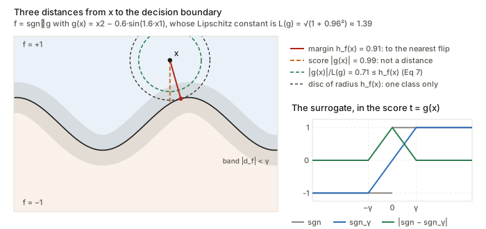
The second term is where the tent of the figure above does its work. The residual |f-F_f|=|\operatorname{sgn}-\operatorname{sgn}_\gamma|\circ d_f=\max(0,1-h_f/\gamma) is a continuous function with values in [0,1], and it is (1/\gamma)-Lipschitz (checks §4). So it concentrates too:
\frac1n\mathbb E\sup_f\sum_i|f-F_f|(x_i)\ \le\ \sup_f\mathbb E|f-F_f| + C_3\frac1\gamma\sqrt{\frac{c\log|\mathcal F|}{nd}}.
Its mean is at most the mass of the band, and isoperimetry on h_f makes that small:
\mathbb E|f-F_f|\le\mathbb P\big(h_f<\tfrac{S(f)}2\big)\le\mathbb P\big(S(f)-h_f>\tfrac{S(f)}2\big)\le e^{-dS(f)^2/(8c)}\le e^{-dS^2/(8c)}.
Adding up gives Eq 5. The paper derives part 2 by pointing to the proof of Theorem 13 “without the \varepsilon-net step”. The three displays above are that proof specialised to a finite class. Widget 3 of the interactive page plots the two parts against \gamma. A small \gamma makes the band cheap and the smooth part expensive, and a large \gamma does the opposite.
App C.1: when does stability help?
Without stability, the residual term can be bounded directly by the maximum of |\mathcal F| sub-Gaussians, giving the Massart-type rate \sqrt{\log|\mathcal F|/n}. Comparing with the middle term of Eq 5:
\frac{\sqrt c}{S}\sqrt{\frac{\log|\mathcal F|}{nd}}\le\sqrt{\frac{\log|\mathcal F|}{n}}\iff S\ge\sqrt{\frac cd}.
So stability improves the bound exactly when the average margin beats the free margin of a random hyperplane. For MNIST-sized d=784 with c=1, the threshold is 0.036 (checks §9).
Corollary 6: the law of robustness for classification
Statement. Under the conditions of Theorem 4.2, let p=\log|\mathcal F|\ge n and \varepsilon,\delta\in(0,1). Suppose the best risk in the class is R^*\ge\varepsilon, and n is large enough that K/\sqrt n<\varepsilon/3 and \sqrt{2\log(2/\delta)/n}<\varepsilon/2. Then with probability at least 1-\delta, for every f\in\mathcal F,
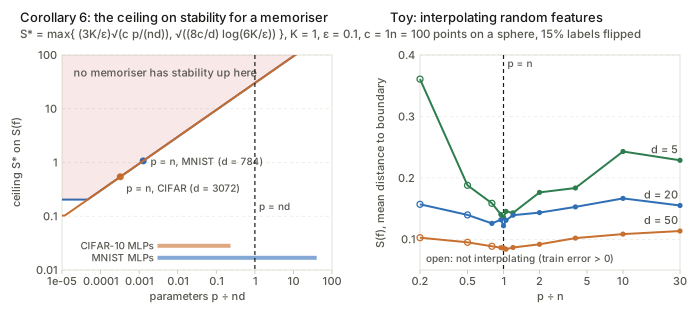
\hat R_{0\text{-}1}(f)\le R^*-\varepsilon\ \Longrightarrow\ S(f)<S_*:=\max\Big\{\frac{3K}{\varepsilon}\sqrt{\frac{c\,p}{nd}},\ \sqrt{\frac{8c}{d}\log\frac{6K}{\varepsilon}}\Big\}. \qquad\text{(Eq 6)}
What the hypothesis means. R^* is the error of the best classifier in the class on fresh data. It is positive when labels are noisy (Remark 7). A classifier with \hat R(f)\le R^*-\varepsilon does better on the training set than any classifier can do on fresh data. It has memorised noise. Interpolation (\hat R=0) is the extreme case.
Proof (App D), in four lines. Let \mathcal F_{S_*}=\{f:S(f)\ge S_*\} be the stable subclass.
- S_* is chosen so that each term of Eq 5 is at most \varepsilon/(3K). For the middle term: \frac{\sqrt c}{S_*}\sqrt{\frac p{nd}}\le\frac{\varepsilon}{3K}\iff S_*\ge\frac{3K}\varepsilon\sqrt{\frac{cp}{nd}}. For the last: 2e^{-dS_*^2/(8c)}\le\frac{\varepsilon}{3K}\iff S_*\ge\sqrt{\frac{8c}d\log\frac{6K}\varepsilon}. Together with K/\sqrt n<\varepsilon/3, this gives \mathcal R(\mathcal F_{S_*})\le\varepsilon/3.
- Eq 1 with Eq 2 and a=1: every stable f has R(f)-\hat R(f)\le\mathcal R(\mathcal F_{S_*})+\varepsilon/2<\varepsilon.
- Since R(f)\ge R^*, every stable f has \hat R(f)>R^*-\varepsilon: no stable classifier memorises.
- Contrapositive: a memoriser is not in \mathcal F_{S_*}, so S(f)<S_*.
Reading the law. The ceiling S_* has two parts. The second, \sqrt{(8c/d)\log(6K/\varepsilon)}, is a floor at the fluctuation scale \sqrt{c/d}. Below it, isoperimetry says nothing, so any margin that small is allowed. The first part grows like \sqrt p:
- At p\approx n it is \frac{3K}\varepsilon\sqrt{c/d}, again of order \sqrt{c/d}. A memoriser with as many parameters as data points has margins no better than the \sqrt{2/(\pi d)} a random hyperplane gets.
- For a memoriser to have margin S at all, it needs p\gtrsim\big(\tfrac{\varepsilon S}{3K}\big)^2\tfrac{nd}{c}. For S of order the data scale, that is p\gtrsim nd: the same overparameterization as Bubeck and Sellke.
Remark 8 notes that nothing here assumes continuity, so quantised networks, spiking networks and attention (which is not globally Lipschitz) are all covered. That is a genuine advantage over Lipschitz-based laws, as long as the class is finite.
Section 5: infinite classes and the co-margin
Why class stability is not enough (Example 9)
For an infinite class the standard move is to cover it by a finite net. Every function is close to some net point, the finite-class bound applies to the net, and closeness takes care of the rest. For this to work, close parameters must give close classifiers. With \operatorname{sgn} in the way, they need not. Take g_w(x)=w\tanh(x) for w\in[-1,1]. For every w\ne0 the classifier has a single boundary point at 0, so its class stability is high. But w=\varepsilon/2 and w=-\varepsilon/2 are \varepsilon apart, and their classifiers disagree at every x\ne0. Class stability says nothing about how far the scores are from zero, and tiny scores flip under tiny parameter changes.
Definition 10 and Eq 7: margins in the output
For f=\operatorname{sgn}\circ g, the co-margin is h^*_g(x)=|g(x)| and the co-stability is S^*(g)=\mathbb E|g|. Both depend on the representation: g and 10g give the same f and different S^* (Remark 11). Dividing by the Lipschitz constant removes that: the normalized co-stability is \bar S^*(g)=\mathbb E|g|/L(g). The link to the input margin is one line. To flip the label, g must travel from g(x) to 0. Since g changes by at most L(g) per unit distance, that takes a distance of at least |g(x)|/L(g):
h_f(x)\ \ge\ \frac{|g(x)|}{L(g)}\quad\Longrightarrow\quad S(f)\ \ge\ \bar S^*(g). \qquad\text{(Eq 7)}
The inequality can be very loose. In the figure above, the wavy score has |g|=0.99 and L(g)=1.39, so the bound is 0.71 while the true margin is 0.91. With a faster wiggle, L(g) grows like the frequency while the margin barely moves (widget 1). Equality holds for the representation g=d_f, where L=1 and |g|=h_f.
Theorem 13: the infinite-class bound
Assumptions. (H3): \mathcal F=\operatorname{sgn}\circ\mathcal G with \mathcal G=\{g_w:\mathcal X\to[-1,1]:\ w\in\mathcal W\}, \mathcal W\subset\mathbb R^p of diameter at most W, and \lVert g_{w_1}-g_{w_2}\rVert_\infty\le J\lVert w_1-w_2\rVert. Every g has S^*(g)>S^* and L(g)\le L, and p\ge n. Then for any covering scale \tilde\varepsilon>0,
\mathcal R_{n,\mu}(\mathcal F)\le K\max\Big\{\frac1{\sqrt n},\ \frac L{S^*}\sqrt{\frac p{nd}}\sqrt{c\log(1+60WJ/\tilde\varepsilon)},\ 2\exp\Big(-\frac{dS^{*2}}{8cL^2}\Big),\ \frac J{S^*}\tilde\varepsilon\Big\}. \qquad\text{(Eq 8)}
Proof (App E), step by step.
- Surrogate. F_{f_w}=\operatorname{sgn}_\gamma\circ g_w with \gamma=S^*(g)/2. It is (L/\gamma)-Lipschitz in x. So is the residual |\operatorname{sgn}\circ g_w-\operatorname{sgn}_\gamma\circ g_w|, because the tent is (1/\gamma)-Lipschitz (Eq 21).
- Net. Take an \tilde\varepsilon-net \mathcal W_{\tilde\varepsilon} of the parameters. Its size is at most (1+60WJ/\tilde\varepsilon)^p, so \log|\mathcal F_{\tilde\varepsilon}|\le p\log(1+60WJ/\tilde\varepsilon). This replaces \log|\mathcal F| in the smooth part, which gives the second term.
- Moving to the net costs little, thanks to the tent. If \lVert w-\tilde w\rVert\le\tilde\varepsilon, the scores differ by at most J\tilde\varepsilon everywhere. The tent is continuous, so the residuals differ by at most J\tilde\varepsilon/\gamma=2J\tilde\varepsilon/S^*. This is the fourth term. With \operatorname{sgn} itself instead of the tent, the difference could be 2, as Example 9 shows.
- Residual at net points. Concentration over the finite net, plus the mean \mathbb E|f-F_f|\le\mathbb P(|g|\le\gamma). Since |g| is L(g)-Lipschitz with mean S^*(g), isoperimetry gives \mathbb P(|g|\le S^*(g)/2)\le2\exp(-dS^*(g)^2/(8cL(g)^2)). That is the third term.
The factor L/S^* plays the role that 1/S played for finite classes (Remark 14): robust predictions need scores that are large relative to how fast they can change.
Corollary 15, and App F
Corollary 15 repeats the argument of Corollary 6. With probability 1-\delta, a classifier that fits below the noise level has
\frac{S^*(g)}{L(g)}<\max\Big\{\frac{3K}\varepsilon\sqrt{\frac p{nd}}\sqrt{c\log(1+60WJ\tilde\varepsilon^{-1})},\ \sqrt{\frac{8c}d\log\frac{6K}\varepsilon}\Big\},
“for all \tilde\varepsilon>0”. Remark 16 asks for W,J polynomial in (n,d,p), so the log is only a log factor. The multi-class extension (App F) runs one-vs-all with the multi-class co-margin g_j(x)-\max_{i\ne j}g_i(x), at the cost of a factor \mathcal C (the number of classes). That multi-class margin is what the experiments measure.
Experiments, in brief
MLPs with 4 or 8 hidden layers and widths 128 to 2048 are trained on MNIST and CIFAR-10 to at least 99% training accuracy. There are also CNNs on CIFAR-10 and Heaviside-activation MLPs on MNIST. S(f) is estimated with Foolbox \ell_2 attacks (DeepFool, PGD) over the radius grid \{0.01,0.05,0.1,0.2,0.5,1,2\}, and L(g) with the ECLipsE estimator. The findings:
- S(f) and \bar S^*(g) grow with width and track test accuracy. For 8-layer CIFAR-10 MLPs, S(f) goes from 0.27 to 0.44 (Fig 1).
- The 8-layer MNIST MLPs show an initial decrease. The authors attribute it to narrow models training for more epochs (7 against 2), and recover the trend with fixed epochs and with widths up to 16384 (Figs 7–9).
- Toy Gaussian data with growing variance break the monotone trend (Fig 4).
How the sizes compare with nd (checks §9, counting weights, biases and batch-norm parameters):
| Setting | nd | smallest model | largest model |
|---|---|---|---|
| CIFAR-10, MLP depth 8 | 1.54\times10^8 | 0.008\,nd (w=256) | 0.23\,nd (w=2048) |
| CIFAR-10, MLP depth 4 | 1.54\times10^8 | 0.003\,nd | 0.12\,nd |
| MNIST, MLP depth 4 | 4.70\times10^7 | 0.003\,nd | 0.30\,nd |
| MNIST, MLP depth 8 | 4.70\times10^7 | 0.005\,nd | 40\,nd (w=16384) |
The largest model in every main-text figure has p<nd.
A toy check: interpolating random features
To see the law act on something I could compute exactly,
rf_margin_toy.py fits a random-features model to n=100 points uniform on the sphere in \mathbb R^d. The sphere is isoperimetric with
c=O(1). Labels are \operatorname{sgn}(x_1) with 15% flipped, so
R^*=0.15. The model is g(x)=a\cdot\operatorname{relu}(Wx)/\sqrt p
with W Gaussian and frozen. For p\ge n, a is
the minimum-norm interpolant. For p<n it is least squares. S(f) is estimated on fresh points by a
DeepFool-style walk to the boundary followed by bisection, so each
distance is an upper bound. At d=20,
averaged over three seeds:
| p/n | 0.2 | 0.5 | 0.8 | 1.0 | 1.2 | 2 | 4 | 10 | 30 |
|---|---|---|---|---|---|---|---|---|---|
| training error | 0.237 | 0.073 | 0 | 0 | 0 | 0 | 0 | 0 | 0 |
| S(f) | 0.157 | 0.140 | 0.126 | 0.122 | 0.139 | 0.143 | 0.153 | 0.167 | 0.155 |
| \lVert a\rVert | 6.1 | 17.1 | 59.6 | 374.5 | 67.1 | 40.0 | 31.4 | 28.6 | 28.0 |
Across dimensions, comparing p=n with p=30n:
| d | S(f) at p=n/5 (not interpolating) | p=n | p=30n | ratio |
|---|---|---|---|---|
| 5 | 0.361 | 0.135 | 0.229 | 1.69 |
| 20 | 0.157 | 0.122 | 0.155 | 1.27 |
| 50 | 0.103 | 0.086 | 0.113 | 1.32 |
Three observations, all consistent with the paper and one qualifying it.
- The least stable interpolant sits at the interpolation threshold p=n. There the fit is forced and \lVert a\rVert peaks (the double-descent spike). More parameters let the minimum-norm solution move the boundary away from the data.
- Margins shrink as d grows, as the \sqrt{c/d} scale predicts, though not as fast as 1/\sqrt d.
- The margin plateaus. With W frozen, the model converges to a fixed kernel interpolant as p\to\infty, so extra parameters stop helping long before the ceiling is reached. The law is a necessary condition. Overparameterization permits stability; it does not produce it. The paper lists sufficiency as open (Sec 7), and this toy is a concrete case where it fails.
- The small, non-interpolating models at p=n/5 have the largest margins. The law only speaks about memorisers.
Eq 7 holds at every p (S(f)\ge the crude bound \mathbb E|g|/(\lVert a\rVert\lVert W\rVert_{op}/\sqrt p)), but that bound is 3–8 times smaller than the measured margin. Widget 5 reruns this in the browser.
Questions and doubts
1. Corollary 15, as stated, loses its dependence on p
Theorem 13 has four terms, the last being J\tilde\varepsilon/S^*, the cost of moving to the net. Corollary 15 keeps only the analogues of the first three, and asserts the implication “for all \tilde\varepsilon>0”. Take \tilde\varepsilon\to\infty. Then \log(1+60WJ/\tilde\varepsilon)\to0, the first term vanishes, and the corollary claims every memoriser has S^*(g)/L(g)<\sqrt{(8c/d)\log(6K/\varepsilon)}, whatever p is. That would make even a model with 10^9 parameters on 6\times10^4 MNIST points unstable. With K=1, \varepsilon=0.1, c=1 the threshold at p=10^9 falls from 459 at \tilde\varepsilon=10^{-3} to 0.204 as \tilde\varepsilon grows, the same as for p=10^5 (checks §10). The fix is to keep the fourth term. Requiring J\tilde\varepsilon/S^*\le\varepsilon/(3K) ties the covering scale to \tilde\varepsilon\le\varepsilon S^*/(3KJ). The log becomes \log(1+180KWJ^2/(\varepsilon S^*)), which Remark 16’s polynomial W,J keep at a log factor. So the conclusion survives, but not as written.
There is a related subtlety. The fourth term needs a lower bound on the unnormalized co-stability S^*(g), but the corollary is phrased through the ratio S^*(g)/L(g). The ratio alone does not rule out Example 9. For g_w=w\tanh x with x\sim\mathcal N(0,1), the ratio is \mathbb E|\tanh x|\approx0.56 for every w\ne0, while S^*(g_w)=0.56|w|\to0 (widget 3b). The corollary should restrict to classes with S^*(g)\ge S^* and state the conclusion for them.
2. Theorem 4.1 is vacuous where it matters, and 4.2 needs fewer assumptions
The paper’s message is about the regime p\approx nd. There Eq 4’s second term is \sqrt c\log|\mathcal F|/(Sn\sqrt d)=\sqrt{cd}/S, which is 28/S for d=784. It is vacuous unless S\gg28 in units where the data have norm about 1 (checks §9). The weakness is the n\log2 from the 2^n subsets. Eq 5 gives \sqrt c/S in the same regime. So Theorem 4.2 carries the paper, and Corollary 6 uses only it.
Theorem 4.2 adds that f^{-1}(1) is closed and \mathcal X path-connected. These are needed only to make d_f Lipschitz. The surrogate F_f=f\cdot\min(1,h_f/\gamma) uses the unsigned margin, which is always 1-Lipschitz. It is (2/\gamma)-Lipschitz with no connectedness at all: if f(x)\ne f(y), then |F_f(x)-F_f(y)|=\min(1,h_f(x)/\gamma)+\min(1,h_f(y)/\gamma)\le2\lVert x-y\rVert/\gamma. Its residual |f-F_f|=\max(0,1-h_f/\gamma) is identical to the one in the paper’s proof. On a finite point cloud, the most disconnected space there is, the measured constants are 2.000/\gamma and 0.974/\gamma (checks §2). As far as I can see, Eq 5 therefore holds under (H1)–(H2) alone, up to a factor of 2 in the constant. The proof sketched above also never uses \log|\mathcal F|\ge n.
3. The experiments do not test the law
Corollary 6 is an upper bound on the stability of memorisers, with an unknown constant K and an unknown isoperimetry constant c for image data. The experiments show that S(f) increases with width. That is consistent with the law, but it would be equally consistent with no law at all. A test would need a memoriser whose stability hits the ceiling, or a measured scaling in p/(nd). The table above also shows that the CIFAR-10 models all have p\le0.23\,nd, and the MNIST models reach nd only at width 16384. The interesting transition is never crossed on CIFAR-10. The Gaussian toy (Fig 4) is where c is known, and there the trend breaks.
4. Heaviside networks and gradient-based attacks
The Heaviside MLPs (Fig 3) report S(f) between 1.6 and 1.88. The attack grid is capped at 2.0, and a failed attack is assigned the cap. A Heaviside network is piecewise constant, with zero gradient almost everywhere. DeepFool and PGD follow gradients, so on such a network they may not move at all unless a surrogate gradient or a decision-based attack is used. The paper does not say which. If attacks mostly failed, the Heaviside curves measure the cap, not the boundary. The attack success rate for these models would settle it.
5. The stability estimates are upper bounds, not “conservative lower bounds”
App G calls the reported stability “conservative lower bounds” because failed attacks are assigned the maximum radius. That misses the main bias. An attack that succeeds at radius r proves the boundary is within r, so every successful estimate is an upper bound on h_f(x). The grid rounds each one up to the next of 7 values, which adds to that. Only the cap pushes the other way. The same holds for my toy (by construction), which is one reason I only compare its values across p, not with any ceiling.
6. Smaller points
- Eq 2 with the absolute value is off by 1/(2\sqrt n), as shown above. Harmless, but the stated equality with C=1/2 is false for the paper’s own definition.
- Notation in App C. The Lipschitz region is defined as A_t(f)=\{h_f>S(f)-t\}, but the partition uses \{h_f\ge S/2\}. These are different sets, and F_f=f on the second is claimed “by construction”. Defining the surrogate on \{h_f\ge S/2\} from the start, as above, fixes it with the same constant 4/S.
- Fact 2 writes a one-sided tail without the factor 2 of Eq 3. That is fine for sub-Gaussian one-sided tails, but it is not what Definition 3 states.
- \gamma depends on w in the proof of Theorem 13 (\gamma=S^*(g)/2), yet step 3 moves between w and a net point as if \gamma were fixed. Using the fixed \gamma=S^*/2 throughout avoids the issue.
- “S(f)>S for every f\in\mathcal F” in Theorem 4 is a strong condition on a whole class. It is harmless only because the corollary applies it to the subclass \mathcal F_{S_*}, which satisfies it by definition.
- d is the ambient dimension in the bounds, while the text appeals to the manifold hypothesis for an intrinsic d. Making that precise needs isoperimetry of the data measure on the manifold, with c relative to the manifold’s own scale. The paper does not attempt it, and the Gaussian toy suggests it matters.
- “Overparameterization is necessary for robustness” is the paper’s slogan. The theorem actually says necessary for memorising while staying robust. A model that does not fit below the noise level is unconstrained. In my toy, the non-interpolating p=n/5 models are the most stable of all.
What would settle it
- A corrected Corollary 15 with \tilde\varepsilon tied to \varepsilon S^*/(3KJ), restricted to S^*(g)\ge S^*.
- An experiment where c is known (the sphere, or a Gaussian at fixed scale) sweeping p through nd at several d, checking whether the largest achievable memoriser margin scales like \sqrt{p/(nd)}.
- Attack success rates for the Heaviside models, and a decision-based attack to cross-check them.
Takeaways
- Replace “Lipschitz constant” with “distance to the boundary” and the Bubeck–Sellke law carries over to classifiers. 2/S plays the role of L, and memorisers need p\gtrsim nd to have margins of order one.
- The scale to compare against is \sqrt{c/d}, the margin a random hyperplane gets for free. Stability helps a bound only above it (App C.1). A memoriser with p\approx n cannot rise much above it (Corollary 6).
- The workhorse is a surrogate: a ramp that is Lipschitz, agrees with the classifier off a thin band, and leaves a tent-shaped residual that is also Lipschitz. Isoperimetry makes the band nearly empty. The same trick handles both the finite and the infinite case.
- For infinite classes the margin must also live in the output. The scores must stay away from zero, or close parameters can give opposite classifiers (Example 9). The normalized co-stability \mathbb E|g|/L(g) is scale-free, but the covering step needs the unnormalized \mathbb E|g|, and Corollary 15 as written loses track of it.
- The law is a ceiling, not a prediction. It says what memorisers cannot do. It does not say that big models will be stable, and a random-features toy shows they need not be.