Provable Guarantees for Self-Supervised Deep Learning with Spectral Contrastive Loss
Links
- arXiv:2106.04156 —
preprint.
make fetchpulls the PDF from here. - NeurIPS 2021 proceedings
- Inequalities and concentration — background page collecting the tools these proofs run on (Cheeger, Donsker–Varadhan, Rademacher, Davis–Kahan and the rest).
Jeff Z. HaoChen, Colin Wei, Adrien Gaidon and Tengyu Ma, Provable Guarantees for Self-Supervised Deep Learning with Spectral Contrastive Loss, NeurIPS 2021.
This is the foundational paper for the augmentation-graph line of analysis. Both Zhang et al. 2026 and the finite-sample machinery reused elsewhere in this repo build directly on it.
In one paragraph
Prior theory for contrastive learning assumed the two views of an example are roughly independent given the label — which is plainly false, since two crops of the same dog are far more alike than two random dogs. This paper drops that assumption entirely and replaces it with a connectivity assumption on a graph. Build the population augmentation graph: vertices are all augmented images, and two are joined if they can be augmentations of the same natural image. Then classes are nearly disconnected components, and within a class there may be sub-graphs (breeds). The paper shows that the minimiser of a simple quadratic loss — the spectral contrastive loss — recovers the top eigenvectors of this graph’s normalised adjacency matrix up to a harmless linear transformation, and that a linear probe on those eigenvectors has error \tilde O(\alpha/\rho_{\lfloor k/2 \rfloor}^2). The bound says something practical: the feature dimension must exceed roughly twice the number of sub-graphs, or the guarantee is vacuous.
The spine of the argument
- Define the population augmentation graph. Connectivity replaces conditional independence.
- Spectral clustering of that graph would give good embeddings — but they are non-parametric, one k-vector per augmented point, and |\mathcal{X}| is exponential.
- Recast eigendecomposition as matrix factorisation, \min \lVert \bar A - FF^\top\rVert_F^2, which decomposes into terms over pairs of rows.
- Reparametrise row x as \sqrt{w_x}\, f(x) for a neural net f. The objective becomes the spectral contrastive loss — a population quantity with an unbiased finite-sample estimator. This is the pivotal move: a global spectral problem becomes a local, sample-based loss.
- Lemma 3.1 says the resulting slack (a diagonal rescaling and an invertible Q) does not affect linear-probe accuracy, so recovering eigenvectors up to that slack is enough.
- Assume few cross-class edges (\alpha small) and that the graph cannot be chopped into many pieces cheaply (\rho_m large for m beyond the sub-graph count). Theorem 3.7 converts these into a linear-probe bound.
- Standard Rademacher concentration lifts the population result to finite samples (Theorems 4.1, 4.2), and margin-free capped-quadratic analysis handles the probe itself (Theorem 5.1).
Setup and notation
| Symbol | Meaning |
|---|---|
| \bar x \sim P_{\bar{\mathcal{X}}} | a natural (un-augmented) data point |
| A(\cdot \mid \bar x) | augmentation distribution |
| \mathcal{X}, N | set of all augmented data and its size; finite but exponentially large |
| y(\bar x) \in [r] | ground-truth label; r downstream classes |
| w_{xx'} | edge weight \mathbb{E}_{\bar x}[A(x\mid \bar x)A(x'\mid\bar x)]; sums to 1 |
| w_x | degree \sum_{x'} w_{xx'} |
| A, D, \bar A | adjacency, degree \operatorname{diag}(w_x), normalised D^{-1/2}AD^{-1/2} |
| \lambda_i, v_i | i-th largest eigenvalue of \bar A and its unit eigenvector |
| F^\star = [v_1,\dots,v_k] | the eigenvector matrix; row u_x^\star is the ideal embedding of x |
| f : \mathcal{X} \to \mathbb{R}^k | the learned encoder; \mathcal{F} its hypothesis class |
| k | representation dimension |
| \mathcal{E}(f) | linear probe error — error of the best linear head on f’s features |
| \alpha | cross-class leakage: labels recoverable from augmentations up to error \alpha (Asm 3.5) |
| \phi_G(S) | Dirichlet conductance of a vertex set S (Def 3.3) |
| \rho_m | sparsest m-partition (Def 3.4) |
| m | number of parts in a partition; morally the number of sub-graphs |
| \hat{\mathcal{R}}_n(\mathcal{F}) | Rademacher complexity of \mathcal{F} on n samples |
| \kappa | uniform bound, \lVert f(x)\rVert_\infty \le \kappa |
| \Delta | eigenvalue gap \lambda_{\lfloor 3k/4\rfloor} - \lambda_k (Thm 4.2) |
Background: reading a graph spectrum
Everything in this paper and its descendants is an argument about the eigenvalues of \bar A. Worth getting the intuition solid before the theorems.
The adjacency matrix is an averaging operator
\bar A is not really a table of numbers; it is an operator. Since (Ax)_i = \sum_j w_{ij} x_j, thinking of a vector as assigning a number to every node, applying A replaces each node’s number with the weighted sum of its neighbours’. For the normalised version it is a genuine average — \bar A is similar to the random-walk matrix D^{-1}A. So \bar A v = \lambda v reads:
this pattern of node-values is reproduced by one round of neighbour-averaging, merely scaled by \lambda.
That single sentence gives the whole interpretation:
- \lambda near 1 — the pattern is smooth along edges; averaging barely changes it. A slow mode: diffusion cannot mix it away.
- \lambda near 0 — the pattern is rough, cancelling across edges; averaging destroys it. A fast mode.
- \lambda negative — averaging flips the pattern; it oscillates across every edge.
Eigenvalues are decay rates under diffusion; eigenvectors are the things decaying.
Reading the spectrum from the top
For a normalised adjacency matrix every eigenvalue lies in [-1,1], and:
- \lambda_1 = 1 always, with eigenvector D^{1/2}\mathbf{1} — essentially the constant function, since averaging a constant returns it. It carries no information; this is the trivial mode one always discards. (It is why Theorem 3.7 needs k \ge 2r rather than k \ge r: one dimension is spent on nothing.)
- The multiplicity of \lambda = 1 counts connected components. Each component supports its own locally-constant eigenvector. So \lambda_2 = 1 exactly iff the graph is disconnected — and \lambda_2 \approx 1 iff it is nearly disconnected, which is exactly Assumption 3.5’s picture of classes.
- 1 - \lambda_2 is the spectral gap, and it measures bottlenecks. Cheeger’s inequality makes this precise: the best possible sparse cut h satisfies \tfrac{1}{2}(1-\lambda_2) \le h \le \sqrt{2(1-\lambda_2)}. Small gap \Leftrightarrow a good cut exists \Leftrightarrow the graph almost falls apart. This is the link between the spectral quantities and the combinatorial \rho_m below.
- \lambda_2’s eigenvector says where to cut (the Fiedler vector): signs give the bipartition, magnitudes give confidence. Points near zero are the ambiguous ones — which is precisely what a boundary example is.
- For m clusters, look at the top m eigenvalues. A clear drop after \lambda_m means m well-separated clusters, and stacking those m eigenvectors as columns embeds each node into \mathbb{R}^m with the clusters pulled apart. That embedding is F^\star.
- The bottom end encodes bipartiteness: \lambda_{\min} = -1 iff a component is bipartite, its eigenvector flipping sign across every edge.
A convention note: the paper’s lemmas use the normalised Laplacian L = I - \bar A, whose eigenvalues are 1 - \lambda_i in [0,2]. “Smallest eigenvectors of L” and “largest of \bar A” name the same objects.
What else a spectrum knows
| Quantity | What it tells you |
|---|---|
| \operatorname{tr}(A^2) | twice the number of edges |
| \operatorname{tr}(A^3) | six times the number of triangles; generally \operatorname{tr}(A^\ell) counts closed walks of length \ell |
| \lambda_1 of unnormalised A | between the average and maximum degree; the effective branching factor, and 1/\lambda_1 is the epidemic threshold |
| top eigenvector of A | eigenvector centrality — the ancestor of PageRank |
| number of distinct eigenvalues | at least \text{diameter} + 1 |
| a localised eigenvector | concentrated on few nodes, signalling a hub or dense subgraph rather than global structure |
The limitation worth knowing: the spectrum is invariant to relabelling, so it is a genuine graph invariant — but not a complete one. Non-isomorphic cospectral graphs exist. The spectrum knows a great deal, not everything.
The picture, on this paper’s own assumptions
Below is a graph built to match Assumption 3.5: r = 3 classes that are nearly disconnected from each other (w \approx 0.0008 across classes), each split into two sub-graphs — think breeds — that are connected to each other only weakly (w = 0.05), with strong connections inside a sub-graph (w = 0.45). Twenty-four augmented points in total.
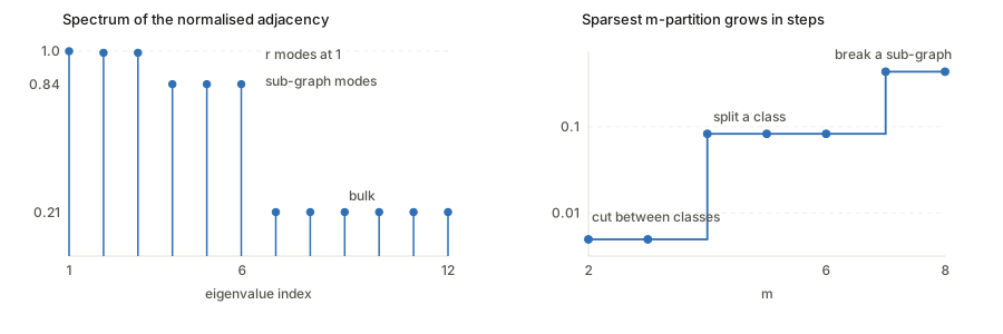
The two panels are the same fact twice, which is what Cheeger’s inequality asserts: flat regions of \rho_m correspond to eigenvalues clustered near 1, and each jump in \rho_m corresponds to a cliff in the spectrum.
Lemma 3.1: why “up to a linear transformation” costs nothing
Statement. For an embedding matrix F \in \mathbb{R}^{N \times k}, a diagonal D with positive entries and an invertible Q \in \mathbb{R}^{k\times k}, set \tilde F = D \cdot F \cdot Q. Then any linear classifier B on F has a counterpart \tilde B = Q^{-1}B on \tilde F making identical predictions, so
\mathcal{E}(F) = \mathcal{E}(\tilde F).
Why it is needed. By Eckart–Young–Mirsky, a minimiser of \lVert \bar A - FF^\top\rVert_F^2 is not the eigenvector matrix itself but
\hat F = F^\star \cdot \operatorname{diag}\big(\sqrt{\lambda_1},\dots,\sqrt{\lambda_k}\big)\, Q
for some orthonormal Q — the factorisation is only determined up to a right rotation, and the eigenvalue scaling comes along too. On top of that, the reparametrisation u_x = \sqrt{w_x}\,f(x) multiplies row x by \sqrt{w_x}, a positive diagonal. So what is actually recovered is the eigenvector matrix pre-multiplied by a positive diagonal and post-multiplied by an invertible matrix. Lemma 3.1 says that is fine.
Why it is true, in one line each.
- Right multiplication by Q. A linear probe computes B^\top u_x. Replacing u_x \mapsto Q^\top u_x and B \mapsto Q^{-1}B leaves B^\top u_x unchanged. The probe simply absorbs Q, and it can, because Q is invertible and the probe is unconstrained.
- Left multiplication by positive diagonal D. This scales each row — each data point’s embedding — by a positive number s_x > 0. Prediction is \arg\max_{i} (B^\top u_x)_i, and scaling a vector by a positive scalar does not change which coordinate is largest. The argmax is scale-invariant.
The conditions matter. Positivity of the diagonal is essential: a negative s_x would flip the argmax. Invertibility of Q is essential: a rank-deficient Q would destroy directions the probe needs.
The caveat. This is about the 0-1 error of the best linear head, nothing more. The rescaling does change margins, norms and the value of any surrogate loss — which is exactly why Theorem 5.1 needs separate work to control the learned probe rather than the best one.
Figure 1 (right): the decomposition of learned representations
The right panel is one equation drawn as matrices. Read it right to left.
\underbrace{\begin{bmatrix} f(x_1)^\top \\ f(x_2)^\top \\ \vdots \end{bmatrix}}_{\text{learned features}} \;\;=\;\; \underbrace{\begin{bmatrix} s_{x_1} \\ s_{x_2} \\ \vdots \end{bmatrix}}_{\text{positive scalars}} \;\odot\; \underbrace{\big[\,v_1 \;\; v_2 \;\; \cdots \;\; v_k \,\big]}_{F^\star,\ \text{top eigenvectors}} \;\cdot\; \underbrace{Q}_{\text{invertible}}
Component by component:
- The rightmost block, “Features”. One row per augmented point, f(x_i)^\top. This is what the network actually outputs after minimising the population spectral contrastive loss. In the figure the rows are bracketed and labelled Brittanys, Beagles, Birmans — the sub-classes, not the downstream classes. That labelling is the point: the structure the features acquire is sub-graph structure.
- The “Eigenvectors” block, F^\star. Columns are v_1, \dots, v_k, the top eigenvectors of \bar A. Row x is the ideal spectral embedding u_x^\star. The figure draws this block with visible sparse vertical bands, and the caption explains why: when sub-classes are exactly disconnected, the eigenvectors are sparse and align with the sub-class structure. Each near-component contributes a near-indicator eigenvector supported on that component — which is the “multiplicity of \lambda=1 counts components” fact from the background section, seen in the eigenvectors rather than the eigenvalues.
- The \odot with the column of s_{x_i}. Row-wise scaling, each row by its own positive scalar. It absorbs both the \sqrt{w_x} from the reparametrisation and the \sqrt{\lambda_i} eigenvalue scaling. The caption stresses s_{x_i} > 0 for every x_i — that is precisely the positivity hypothesis Lemma 3.1 needs.
- The Q block. An arbitrary invertible mixing of the k coordinates. The network has no reason to output the eigenvectors in any particular basis, and this is the freedom the factorisation leaves. Lemma 3.1 makes it harmless.
What the figure is arguing. The learned representation is not approximately spectral and not inspired by spectral clustering. It is exactly the spectral embedding, composed with two transformations that a linear probe cannot see. So any statement provable about spectral clustering transfers to the trained network — which is the licence for the whole rest of the paper.
Two practical readings follow. Individual coordinates of f(x) are not interpretable, because Q scrambles them arbitrarily; only the span is determined. And the norm \lVert f(x)\rVert carries s_x, i.e. graph degree information, not semantics — one reason practitioners normalise features before use and lose nothing by it.
Dirichlet conductance and sparsest m-partition
These two definitions are how the paper converts “the data is continuous within a class” into something a theorem can consume.
Dirichlet conductance (Def 3.3). For a vertex set S,
\phi_G(S) := \frac{\sum_{x \in S,\, x' \notin S} w_{xx'}}{\sum_{x\in S} w_x}
— of all the edge weight touching S, what fraction leaves? It is a leakage rate, in [0,1]. Near 0 means S is nearly a closed component; near 1 means S is barely held together relative to its outside connections. The paper notes the degenerate case: for a singleton \{x\}, \phi_G = 1, because w_x counts the self-loop too. Singletons are maximally leaky, which matters below.
Sparsest m-partition (Def 3.4).
\rho_m := \min_{S_1,\dots,S_m} \max\{\phi_G(S_1),\dots,\phi_G(S_m)\}
over partitions of \mathcal{X} into m non-empty parts. The \max inside asks for the worst (leakiest) part — so no part is allowed to be a bad cluster — and the \min outside picks the best such partition. So: \rho_m is the cost of the cheapest way to break the graph into m decent pieces.
Reading the two quantifiers in the right order is the whole trick. \rho_m small means a good m-way split exists. \rho_m large means every m-way split has at least one badly leaky part — the graph refuses to be cut that finely.
How they enter the theorems. The bound is \mathcal{E}(f^\star_{\text{pop}}) \le \tilde O(\alpha/\rho_{\lfloor k/2\rfloor}^2), so a large \rho_{\lfloor k/2\rfloor} is what makes the guarantee good. The logic:
- \rho_r \approx 0 — augmentations from different classes nearly form a disjoint r-way partition, so cutting along class boundaries is almost free. This is not used as the good case; it is the statement that class structure exists.
- For m > r we want \rho_m large. If a class contains t well-connected sub-graphs, any (t+1)-way partition must split one sub-graph, incurring constant conductance. So \rho_{t+1} = \Omega(1).
- The bound uses m = \lfloor k/2\rfloor. Raising k lets you invoke a larger m, and larger m means larger \rho_m, hence a better bound. That is the mechanism behind the dimension requirement: k must be big enough that \lfloor k/2\rfloor exceeds the number of sub-graphs.
- The singleton fact caps the whole thing usefully: \rho_N = 1, so \rho_m increases to 1 and there is nothing to gain past m = N.
On the toy graph in the figure above (r=3, six sub-graphs), the bound multiplier 1/\rho_{\lfloor k/2\rfloor}^2 behaves like this:
| k | \lfloor k/2 \rfloor | \rho_{\lfloor k/2\rfloor} | bound \approx |
|---|---|---|---|
| 6 | 3 | 0.0050 | 40{,}000\,\alpha — vacuous |
| 8 | 4 | 0.0830 | 145\,\alpha |
| 12 | 6 | 0.0830 | 145\,\alpha |
| 14 | 7 | 0.4342 | 5.3\,\alpha |
A 7500-fold improvement from k=6 to k=14, and the jumps land exactly where the partition is forced to start breaking sub-graphs. This is why the paper’s headline advice — representation dimension must exceed roughly twice the number of sub-graphs — is a real prediction rather than a technical artefact.
Theorem 3.7, broken down
Statement. Assume k \ge 2r and Assumption 3.5 holds with parameter \alpha > 0. Let \mathcal{F} satisfy realizability (Asm 3.6) and let f^\star_{\text{pop}} \in \mathcal{F} minimise the population spectral contrastive loss. Then
\mathcal{E}(f^\star_{\text{pop}}) \;\le\; \tilde O\!\left(\frac{\alpha}{\rho_{\lfloor k/2\rfloor}^2}\right).
Four pieces, each worth reading on its own.
The quantity being bounded, \mathcal{E}(f). Not the training loss, and not the error of some particular classifier: the error of the best possible linear head on the learned features (Eq. 1). So the theorem is a statement about linear separability of the representation — are the classes linearly recoverable at all. It says nothing yet about whether a learned probe finds that head; Theorem 5.1 handles that.
The numerator \alpha: how much the classes leak. Assumption 3.5 says some classifier recovers y(\bar x) from a single augmentation x with error at most \alpha. Equivalently, two examples from different classes can rarely be augmented to the same point — few cross-class edges. Error is proportional to \alpha, which gives the clean limiting case the paper highlights: if \alpha = 0, the bound is zero and recovery is exact. So the theorem degrades gracefully rather than having a floor. Note \alpha is a property of the augmentation strength, not of k: too-aggressive augmentation that blends cats into dogs raises \alpha irreducibly.
The denominator \rho_{\lfloor k/2\rfloor}^2: how stubbornly connected the graph is. From the previous section, large is good, and k buys you a larger index. The square is a Cheeger-type artefact — conductance controls spectral gaps only up to squaring, so the quadratic dependence is the usual price of going from combinatorics to spectra, not a statement about the data. The foundations page checks numerically just how loose that direction is.
Why k \ge 2r and not k \ge r. Two dimensions are spent on overhead. One goes to the trivial eigenvector \lambda_1 = 1, which carries no information. The rest is the analysis needing room beyond the bare r class directions to linearly separate them — the appendix generalises \lfloor k/2\rfloor to any constant fraction of k, which says the factor 2 is a proof convenience rather than a sharp threshold.
How to read it overall. Error \lesssim (how much classes bleed together) / (how hard the graph is to over-partition)². The numerator is set by your augmentation pipeline; the denominator by the data’s intrinsic connectivity and your choice of k. The only knob is k, and the theorem says: make it comfortably larger than twice the number of distinct sub-populations you believe exist.
What it does not say. Nothing about optimisation — f^\star_{\text{pop}} is assumed to be a global minimiser, via Assumption 3.6. Nothing about whether SGD finds it. And \rho_{\lfloor k/2\rfloor} is not computable for real data, so the bound is explanatory, not a number you can evaluate. Section 3.4 partly answers this by instantiating it on a mixture of manifolds (Example 3.8, Theorem 3.9), where \rho_{\lfloor k/2\rfloor} \gtrsim \sigma/\sqrt d and the whole bound becomes \tilde O(1/(\sigma^2 \cdot \text{poly}(d))) — non-trivial even when the augmentation noise \sigma is polynomially small, i.e. much weaker than the data scale.
Finite-sample generalization bounds
Section 3 is entirely about the population loss. Sections 4 and 5 close the three gaps between that and a real pipeline. It is worth naming them separately, because the paper’s guarantee is a chain and each link is a different theorem.
Gap 1: finite unlabeled data → population loss (Theorem 4.1)
The empirical loss \hat{\mathcal{L}}_n(f) (Section 4) is an unbiased estimator of \mathcal{L}(f) — this is why the quadratic form matters, and it is where the spectral loss decisively beats InfoNCE, whose batch denominator makes it biased at finite batch size. The negative-pair term uses the n(n-1) distinct ordered pairs i \ne j precisely to keep it unbiased.
Given that, ordinary uniform convergence applies. With \lVert f(x)\rVert_\infty \le \kappa and \hat f_{\text{emp}} minimising the empirical loss, with probability 1-\delta:
\mathcal{L}(\hat f_{\text{emp}}) \;\le\; \mathcal{L}(f^\star_{\text{pop}}) + c_1 \hat{\mathcal{R}}_{n/2}(\mathcal{F}) + c_2\sqrt{\frac{\log 2/\delta}{n}},
with c_1 \lesssim k^2\kappa^2 + k\kappa and c_2 \lesssim k\kappa^2 + k^2\kappa^4. Read the constants: they grow polynomially in k and \kappa, because the loss involves products of two k-dimensional bounded vectors, so the effective range scales like k\kappa^2 and the squared term like k^2\kappa^4. Rademacher complexity \hat{\mathcal{R}}_n(\mathcal{F}) is extended to vector outputs by taking the worst coordinate. Plug in any off-the-shelf bound for your architecture; the paper does ReLU nets in Section E.2.
Gap 2: near-optimal loss → near-optimal linear probe (Theorem 4.2)
Theorem 4.1 gives a small excess loss \epsilon, not a small error. Getting from one to the other is genuinely non-trivial: a tiny loss perturbation could in principle rotate the learned subspace a lot, if the eigenvalues involved are nearly tied. So a spectral gap condition appears. Assuming k \ge 4r+2 and \mathcal{L}(\hat f_{\text{emp}}) < \mathcal{L}(f^\star_{\text{pop}}) + \epsilon with \epsilon < \Delta/k^2:
\mathcal{E}(\hat f_{\text{emp}}) \;\lesssim\; \frac{\alpha}{\rho_{\lfloor k/2\rfloor}^2}\log k \;+\; \frac{k\epsilon}{\Delta}, \qquad \Delta := \lambda_{\lfloor 3k/4\rfloor} - \lambda_k .
The first term is Theorem 3.7. The second is the price of imperfect optimisation, and it is linear in \epsilon — the reassuring conclusion, since it means no catastrophic amplification. But it is divided by \Delta: if the eigenvalues between indices 3k/4 and k are bunched together, the learned subspace is ill-determined and the penalty blows up. This is standard eigenspace perturbation (Davis–Kahan in spirit) surfacing in the bound. Note k \ge 4r+2, stricter than Theorem 3.7’s k \ge 2r: the room between 3k/4 and k has to exist for \Delta to be meaningful.
Gap 3: best linear probe → learned linear probe (Theorem 5.1)
Theorem 3.7 promises a good linear head exists. Fitting one from labelled data is another matter, and the obstacle the paper flags is honest: a 0-1 error guarantee says nothing about the margin, so margin-based generalisation theory cannot be invoked. Their fix is to sidestep margins entirely and fit a capped quadratic loss,
\ell((z, y), B) := \sum_{i=1}^{r} \min\Big\{\big(B^\top z - \vec y\big)_i^2,\, 1\Big\},
with \vec y the one-hot label. Capping bounds the loss so concentration applies. With a norm constraint \lVert B\rVert_F \le 1/C and n labelled examples:
\Pr\big[\bar g_{f^\star,\hat B}(\bar x) \ne y(\bar x)\big] \;\lesssim\; \frac{\alpha}{\rho_{\lfloor k/2\rfloor}^2}\log k \;+\; \frac{r}{C}\sqrt{\frac{k}{n}} \;+\; \sqrt{\frac{\log 1/\delta}{n}}.
First term: the population error from Theorem 3.7. Last two: ordinary \sqrt{k/n} generalisation gap for linear classification. The paper’s own observation is the one to keep: this exposes a trade-off in k. Larger k shrinks the first term (bigger \rho_{\lfloor k/2\rfloor}) but grows the third (more parameters to fit from n labels). So k should be large but not unboundedly so — and unlike the population theory, which always prefers bigger k, the full chain has an interior optimum. The stated difficulty of the proof is exhibiting a small-norm B with small population quadratic loss, which does not follow from a 0-1 guarantee.
The chain, assembled. Minimise the empirical spectral loss on n unlabeled samples (Thm 4.1 → small excess loss \epsilon) → features are nearly the top eigenvectors (Thm 4.2 → linear probe error \approx population value +\, k\epsilon/\Delta) → fit a capped-quadratic probe on labelled data (Thm 5.1 → learned probe error +\,O(\sqrt{k/n})). Sample complexity is polynomial in the Rademacher complexity, k, \kappa and 1/\Delta throughout.
Questions and doubts
- \rho_m is not estimable. The whole guarantee is parametrised by a quantity requiring a minimum over all m-way partitions of an exponentially large graph — NP-hard even to approximate well in general. Section 3.4 instantiates it for one synthetic family; for real image data the bound cannot be evaluated, only believed.
- The factor-of-2 in \lfloor k/2\rfloor is soft. The appendix relaxes it to any constant fraction, which means the “k must exceed twice the sub-graph count” headline is really “k must exceed a constant multiple”, with the constant unpinned.
- Realizability (Asm 3.6) is strong and load-bearing. It assumes a global minimiser of the population loss lies in \mathcal{F}. The paper notes it can be relaxed to approximate realizability at the cost of an extra term, but the size of that term for real networks is not characterised. No optimisation analysis anywhere.
- The augmentation graph is a population object over an exponentially large vertex set. Whether finite-sample empirical graphs approximate its spectrum is not addressed; the finite-sample results concern the loss, and route around the graph rather than approximating it.
- \Delta in Theorem 4.2 could plausibly be tiny. For a graph whose spectrum has a long flat bulk — which is exactly what the toy example and the Zhang paper’s construction both exhibit — \lambda_{\lfloor 3k/4\rfloor} - \lambda_k \approx 0 and the k\epsilon/\Delta term dominates everything. The paper does not discuss when \Delta is safely bounded away from zero.
- Assumption 3.5’s \alpha conflates two things: genuinely ambiguous images, and over-aggressive augmentation. Both raise \alpha, but only the second is under the practitioner’s control, and the theory cannot separate them.
Takeaways
- The conceptual contribution outlasts the bounds: contrastive learning is spectral clustering of the augmentation graph, exactly and not by analogy, and the bridge is the matrix-factorisation identity plus Lemma 3.1.
- Replacing conditional independence with graph connectivity is the right move. It matches what augmentations actually do, and it accommodates sub-classes — downstream labels need only be a coarsening of the sub-graph partition, not aligned with it.
- The actionable prediction is the dimension requirement: k must exceed a constant multiple of the number of distinct sub-populations, not the number of downstream classes. This explains why practitioners find large projection dimensions help on diverse data.
- Theorem 5.1 exposes a genuine trade-off in k that the population theory hides: bigger k improves the representation but costs labelled-sample efficiency in the probe.
- The quadratic repulsion is not just analytically convenient — it makes the empirical loss an unbiased estimator of the population loss, which is what lets standard concentration close the finite-sample gap. That is a concrete advantage over InfoNCE, and the experiments report comparable accuracy to SimCLR without needing large batches.