Integral probability metrics: a panel of judges (TV, Wasserstein-1, Dudley, MMD)
Links
- Interactive
version: drag a ramp judge over two densities and watch the
gap it earns, the area-between-CDFs picture, and the best judge of any
shape; plot TV, Dudley, W_1, KL and a
Gaussian-kernel MMD against the separation of two Gaussians or of two
point masses; draw the MMD witness function for two samples and slide
the kernel bandwidth. On load the page recomputes 45 numbers from
ipm.pyand reports its largest deviation. - Runnable
code: every number on this page, and the four figures
(
python3 ipm.py --figures). numpy and the standard library only.make verifyruns it. - Read first, if you want the picture behind W_1: Optimal transport (the Kantorovich–Rubinstein duality of its §7 is the W_1 case of this page). For kernels and the “Hilbert space” vocabulary see HSIC §3 and §5: HSIC is an MMD between the joint distribution and the product of its marginals.
- A paper that leans on this: Tahir, Ganguli & Rotskoff 2025, Features are fate. Its Appendix A lower-bounds a Dudley distance with a single well-chosen judge and notes that the result carries over to W_1; §10 below checks that argument.
- References: B. K. Sriperumbudur, K. Fukumizu, A. Gretton, B. Schölkopf & G. R. G. Lanckriet, On integral probability metrics, \varphi-divergences and binary classification, arXiv:0901.2698 (2009): the reference used here. A. Müller, Integral probability metrics and their generating classes of functions, Adv. Appl. Probab. 1997 (the name). R. M. Dudley, Real Analysis and Probability, 2002, ch. 11 (the bounded Lipschitz metric). A. Gretton et al., A kernel two-sample test, JMLR 2012 (MMD as a test). The three citations after the first are from memory.
In one paragraph
How far apart are two distributions P and Q? Ask a judge. A judge is a function h that gives every possible outcome a score. Average the score over draws from P, do the same for Q, and compare the two averages: the gap says how well this one judge can tell P from Q. An integral probability metric (IPM) is the gap of the best judge in a fixed panel \mathcal F: \gamma_{\mathcal F}(P,Q)=\sup_{h\in\mathcal F}\lvert\mathbb E_Ph-\mathbb E_Qh\rvert. The whole content is the choice of panel. Any judge with scores between 0 and 1 gives total variation. Judges that may not slope steeper than 1 give the Wasserstein-1 (earth mover’s) distance. Judges whose height plus steepness is at most 1 give the Dudley (bounded Lipschitz) distance. The unit ball of a kernel’s function space gives MMD. Unlike KL and the other \varphi-divergences, which compare the two probability tables point by point and explode when the supports do not overlap, an IPM with a bounded panel is always finite, and one with smooth judges notices how far the mass has moved. The price is that a panel must be chosen: two distributions can be far apart for one panel and identical for another, and the panel is never the downstream task. This page works out the simplest cases in closed form and checks every number a second way.
1. Symbols
| Symbol | Read it as |
|---|---|
| P,\;Q | two probability distributions on the same space \mathcal X: say the distribution of one embedding coordinate under two data sets |
| p,\;q and F,\;G | their densities, and their CDFs F(x)=P(X\le x), G(x)=Q(Y\le x) |
| h:\mathcal X\to\mathbb R | a judge: a score for every outcome |
| \mathbb E_Ph | the average of h over draws from P: \sum_xP(x)h(x) for a table, \int h(x)p(x)\,dx for a density, the sample mean for a data set |
| \mathcal F | the panel: the set of judges allowed |
| \sup | “supremum”: the largest value, or the value the largest ones approach |
| \gamma_{\mathcal F}(P,Q) | the IPM for panel \mathcal F: the best judge’s absolute gap |
| d(x,y) | the ground distance between two outcomes (Euclidean distance between embeddings, say) |
| \lVert h\rVert_\infty=\sup_x\lvert h(x)\rvert | how tall the judge is |
| \lVert h\rVert_L=\sup_{x\ne y}\lvert h(x)-h(y)\rvert/d(x,y) | how steep the judge is: its Lipschitz constant |
| \lVert h\rVert_{BL}=\lVert h\rVert_L+\lVert h\rVert_\infty | height plus steepness, the Dudley “budget” |
| \mathrm{TV},\;W_1,\;\gamma_\beta,\;\mathrm{MMD} | total variation, Wasserstein-1, Dudley’s bounded Lipschitz distance, maximum mean discrepancy |
| \delta_x | a point mass: all the probability sits at the single outcome x |
| k(x,y), \mathcal H_k, \mu_P | a kernel (a similarity between outcomes), its function space, and the average of k(x,\cdot) under P (§7) |
2. A panel of judges
Four bins. Cut one embedding coordinate into four bins and count how often each occurs among samples from P and from Q:
| bin | 1 | 2 | 3 | 4 |
|---|---|---|---|---|
| P | 0.5 | 0.3 | 0.2 | 0.0 |
| Q | 0.2 | 0.3 | 0.1 | 0.4 |
A judge is one number per bin. Take h=(0,0,0,1), “score 1 if the sample lands in bin 4”. Its average score is 0.0 under P and 0.4 under Q: a gap of 0.4. Take h=(1,0,1,0): the averages are 0.7 and 0.3, again a gap of 0.4. The constant judge (1,1,1,1) earns a gap of 0 whatever P and Q are, because it scores every outcome alike. Which judge is best depends on which judges are allowed. That is the whole idea:
\gamma_{\mathcal F}(P,Q)\;=\;\sup_{h\in\mathcal F}\;\Big\lvert\,\mathbb E_{x\sim P}\,h(x)\;-\;\mathbb E_{y\sim Q}\,h(y)\,\Big\rvert .
Some things follow at once.
- Different panels, different metrics. Every distance in this page is this formula with a different \mathcal F; §8 tabulates them.
- The absolute value is free whenever the panel contains -h along with h (the Lipschitz, Dudley and MMD panels), or 1-h (the [0,1] panel): flipping the judge flips the sign of the gap. The half-line panel of §3 is the exception, since F-G can change sign.
- Bigger panel, bigger sup. If \mathcal F\subseteq\mathcal F' then \gamma_{\mathcal F}\le\gamma_{\mathcal F'} (§10 uses this).
- A panel can be too small. With \mathcal F=\{h(x)=x\} the “best judge” only sees the means, so two different distributions with equal means are at distance 0. A panel rich enough that \gamma=0 forces P=Q is called characteristic (or separating). The panels of §§3–7 are (for MMD, with a Gaussian kernel); the one-function panel above is not.
- The best judge is informative. It is the function that separates P from Q most, so looking at it shows where they differ. The WGAN critic and the MMD witness (§7) are exactly this.
Sriperumbudur et al. also connect \gamma_{\mathcal F} to binary classification, through the optimal risk of a classifier drawn from the panel (their abstract). So an IPM is also “how well can a classifier of this type tell P from Q”. I did not check the precise statement.
3. Total variation: judges scored between 0 and 1
Score every outcome between 0 and 1. Then
\mathbb E_Ph-\mathbb E_Qh=\int h(x)\,\big(p(x)-q(x)\big)\,dx
is largest when h=1 exactly where p>q and h=0 elsewhere: the judge collects the whole positive part of p-q and none of the negative part. The result is \int_{p>q}(p-q)=\tfrac12\int\lvert p-q\rvert=\mathrm{TV}(P,Q) (the positive and negative parts of p-q have equal size, since p and q both integrate to 1). A judge that scores 0 or 1 is the indicator of a set A, and its gap is \lvert P(A)-Q(A)\rvert, so equivalently \mathrm{TV}=\sup_A\lvert P(A)-Q(A)\rvert: “the largest probability difference of any event”. If judges may range over [-1,1] instead, the result doubles to \int\lvert p-q\rvert=2\,\mathrm{TV}.
On the four bins: \tfrac12\sum\lvert p_i-q_i\rvert=0.4. The best set is \{p>q\}=\{1,3\}, with P(A)=0.70 and Q(A)=0.30. Ties are possible: the sets \{4\}, \{1,3\}, \{2,4\} and \{1,2,3\} all reach 0.4. Among 200000 random judges with scores in [0,1] the best gap is 0.3959, never above 0.4, and the judge \operatorname{sign}(p-q) with scores in [-1,1] earns 0.8=2\,\mathrm{TV}.
Kolmogorov distance is the panel of half-line indicators h_t(x)=\mathbf 1[x\le t], whose gap is \lvert F(t)-G(t)\rvert, so \sup_t\lvert F-G\rvert. It needs an ordering of the outcomes, so it lives on the line. It is at most TV (half-lines are special sets); on the four bins it equals 0.4.
What TV cannot see. It only asks whether the mass is in the same place, not how far it moved. Two point masses \delta_0 and \delta_D have \mathrm{TV}=1 for D=0.1 and D=100 alike (§5.1).
4. Lipschitz judges: Wasserstein-1
Now let a judge score anything, but forbid it from changing faster than the ground distance: \lvert h(x)-h(y)\rvert\le d(x,y), i.e. \lVert h\rVert_L\le1. Then
W_1(P,Q)=\sup_{\lVert h\rVert_L\le1}\ \mathbb E_Ph-\mathbb E_Qh
is the Kantorovich–Rubinstein duality: the largest gap of a 1-Lipschitz judge equals the cost of the cheapest way to reshape P into Q (Optimal transport §§1, 7). The best judge is the WGAN critic. Two immediate consequences:
- The judge h(x)=x is 1-Lipschitz, so W_1\ge\lvert\mu_P-\mu_Q\rvert: shifting a distribution by m moves it at least m in W_1. In the embedding picture, P=N(0,I) in \mathbb R^2 and Q = P shifted by 3 along the first coordinate: the judge h(z)=z_1 earns exactly 3.0000, and moving every point by (3,0) is a valid reshaping of cost 3, so W_1=3.
- No sup-norm bound is imposed, so W_1 has no ceiling. It grows with the separation.
In one dimension it is an area. For a judge with derivative h', integration by parts gives
\mathbb E_Ph-\mathbb E_Qh=\int h(x)\,d(F-G)(x)=\int h'(x)\,\big(G(x)-F(x)\big)\,dx .
The boundary terms vanish because F-G\to0 at both ends and h is bounded (for an unbounded 1-Lipschitz h the two distributions need finite first moments). In words: a judge earns money only where it tilts (h'\neq0), and where it tilts it earns the slope times G-F, the amount by which Q has more mass to the left of x than P has. Choose the slope with the sign that makes each term positive, h'=\operatorname{sign}(G-F), and
W_1(P,Q)=\int\lvert F(x)-G(x)\rvert\,dx ,
the area between the two CDFs. This is the same as the sort-and-match rule of the optimal transport page. The code checks all three routes on n=60 samples each of N(0,1) and N(1,1): sorted samples \tfrac1n\sum_i\lvert x_{(i)}-y_{(i)}\rvert=0.962085, the area between the empirical CDFs =0.962085, and a Hungarian-algorithm assignment =0.962085 (on the second seed 1.064313 for the sorted formula and for the assignment). A random pairing costs 1.3661. The Hungarian potentials also give the dual judge explicitly: it has largest slope 1.0000 between the 120 sample points and earns 0.962085. The value equals the difference of the sample means (0.962085) because every sorted pair has y_{(i)}>x_{(i)}; the population value for these Gaussians is W_1=1.
5. A judge with a budget: the Dudley metric
W_1 lets a judge be arbitrarily tall, so it can be enormous when a distribution has far outliers. Cap the sum of height and steepness instead:
\gamma_\beta(P,Q)=\sup_{\lVert h\rVert_L+\lVert h\rVert_\infty\le1}\ \lvert\mathbb E_Ph-\mathbb E_Qh\rvert .
The budget of 1 is spent on two things: a on height, L=1-a on steepness. A tall judge must be gentle, a steep one must be short. (Some texts use \max(\lVert h\rVert_L,\lVert h\rVert_\infty)\le1; both metrise the same notion of convergence, but the numbers differ. This page uses the sum, as Dudley and Tahir et al. do.) Three facts follow from the panel being inside two others:
- Every such h is 1-Lipschitz, so \gamma_\beta\le W_1.
- Every such h has \lvert h\rvert\le1, so \gamma_\beta\le2\,\mathrm{TV}\le2: the metric cannot exceed 2 however far apart the distributions are.
- It metrises weak convergence on separable metric spaces (Dudley; I cite it, I do not re-derive it).
5.1 Two point masses, in closed form
Let P=\delta_0, Q=\delta_D. Then the gap of any judge is \lvert h(0)-h(D)\rvert. Under the budget (a,\,L=1-a) that difference is at most \min(2a,\;LD): the two values both lie in [-a,a], and they are D apart, so they differ by at most L times D. The first term rises with a, the second falls; they are equal when 2a=(1-a)D, i.e. a=D/(D+2) and L=2/(D+2), and the common value is
\gamma_\beta(\delta_0,\delta_D)=\frac{2D}{D+2}.
| D | \mathrm{TV} | W_1=D | Dudley 2D/(D+2) | \mathrm{KL}(P\Vert Q) | Gaussian-kernel MMD, bandwidth 1 |
|---|---|---|---|---|---|
| 0.1 | 1 | 0.1 | 0.0952 | \infty | 0.0999 |
| 1 | 1 | 1 | 0.6667 | \infty | 0.8871 |
| 2 | 1 | 2 | 1.0000 | \infty | 1.3150 |
| 5 | 1 | 5 | 1.4286 | \infty | 1.4142 |
| 100 | 1 | 100 | 1.9608 | \infty | 1.4142 |
A grid search over a agrees with the closed form to within 10^{-5} at every D in the table. The ratio Dudley/W_1=2/(D+2) is 0.9950 at D=0.01 and 0.0196 at D=100: the Dudley distance is the Wasserstein distance for tiny D and saturates at 2 for large D. TV is blind to D throughout, KL is infinite throughout. For D=2, the Dudley and TV values coincide at 1.
5.2 A ramp reads an area
Restrict to ramp judges, h(x)=\operatorname{clip}\big(L(x-c),\,-a,\,a\big): flat at -a, then climbing with slope L around the centre c, then flat at +a. The sloping part is a window of length 2a/L. By the integration-by-parts formula of §4, the gap of a ramp is
\lvert\mathbb E_Ph-\mathbb E_Qh\rvert=L\,\bigg\lvert\int_{\text{window}}(G-F)\,dx\bigg\rvert ,
that is, L times the area between the two CDFs, over the ramp’s window. The code checks it three ways for P=N(0,1), Q=N(1,1), a=0.6, L=0.4, c=0.5: a closed form for the expectation of a clipped Gaussian gives 0.340140, numerical integration of \int h(p-q) gives 0.340140, and L\times the area of F-G over the window [-1,2] (=0.850350) gives 0.340140.
Two limits. Widen the window to the whole line with L=1: the ramp is a straight line and its gap is \lvert\mu_P-\mu_Q\rvert=\lvert\int(G-F)\rvert. That equals W_1=\int\lvert F-G\rvert when F-G never changes sign, as for the shift pair, and is smaller otherwise. Shrink the window to a point and the ramp becomes a step of height a on either side, which measures 2a\,\lvert F(c)-G(c)\rvert, the Kolmogorov distance. The Dudley budget forces a trade-off in between: \text{gap}(a)=(1-a)\,A\big(2a/(1-a)\big), where A(w) is the largest (signed) area between the CDFs that a window of length w can capture, and \gamma_\beta is the maximum over a.
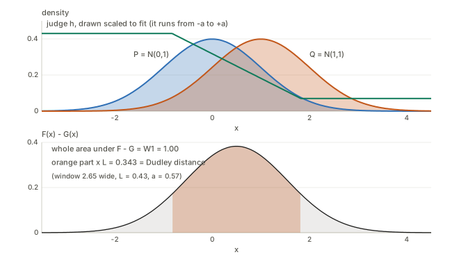
Why a ramp is the best judge here. Take the shift pair, where \Delta=F-G\ge0 is a single hump, symmetric about c=m/2. By the formula of §4 the gap is \int(-h')\,\Delta\,dx. Write \Delta as a stack of layers, \Delta(x)=\int_0^\infty\mathbf 1[\Delta(x)>t]\,dt. Each layer \{\Delta>t\} is an interval I_t=(l_t,r_t) centred at c, and \int_{I_t}(-h')=h(l_t)-h(r_t), so
\text{gap}=\int_0^\infty\big(h(l_t)-h(r_t)\big)\,dt\ \le\ \int_0^\infty\min\big(2a,\;L\,\lvert I_t\rvert\big)\,dt ,
because two values of a judge with \lvert h\rvert\le a differ by at most 2a, and by at most L times their distance. The decreasing ramp centred at c meets the bound with equality for every layer, so no judge of any shape does better. This argument needs the symmetric hump. For a multi-humped F-G a ramp is only a lower bound, as §6 shows; for a single asymmetric hump I do not know.
5.3 Gaussians moved apart
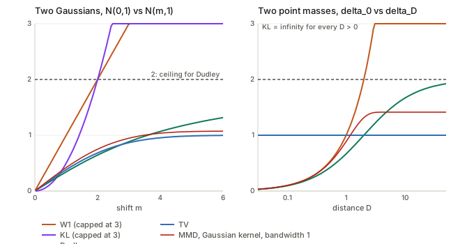
For N(0,1) against N(m,1) the standard formulas are \mathrm{KL}=m^2/2, W_1=\lvert m\rvert, \mathrm{TV}=2\Phi(\lvert m\rvert/2)-1 (with \Phi the standard normal CDF), and the Kolmogorov distance equals TV because the CDF gap peaks at m/2. The Dudley value comes from the ramp window formula, using the antiderivative \int\Phi(z)dz=z\Phi(z)+\varphi(z) (\varphi the normal density):
| m | \mathrm{KL}=m^2/2 | W_1 | \mathrm{TV} | Dudley | best a |
|---|---|---|---|---|---|
| 0.5 | 0.1250 | 0.5 | 0.1974 | 0.1743 | 0.564 |
| 1 | 0.5000 | 1 | 0.3829 | 0.3427 | 0.570 |
| 2 | 2.0000 | 2 | 0.6827 | 0.6438 | 0.590 |
| 4 | 8.0000 | 4 | 0.9545 | 1.0684 | 0.657 |
| 8 | 32.0000 | 8 | 0.9999 | 1.4688 | 0.771 |
A search over the ramp family with the closed-form Gaussian expectation gives the same Dudley values to four decimals (1.0684 against 1.0683 at m=4, the grid resolution), with centre c=m/2 every time. TV saturates at 1, Dudley creeps towards 2 but at m=8 is only 1.4688, W_1 grows without limit, and KL grows quadratically. Pinsker’s inequality \mathrm{TV}\le\sqrt{\mathrm{KL}/2} holds (0.3829\le0.5000 at m=1); the reverse is impossible, since TV never exceeds 1.
5.4 “Like W_1 for close distributions” needs a scale
A common description is that Dudley behaves like W_1 when the distributions are close and like TV when they are far. The far half is right up to a factor: Dudley tends to 2=2\,\mathrm{TV}. The close half is true only for narrow distributions. For N(0,s^2) against N(m,s^2) with m\to0, the ratio Dudley/W_1 tends to a constant that depends on s:
| width s | 2 | 1 | 0.3 | 0.1 | 0.03 | 0.01 |
|---|---|---|---|---|---|---|
| Dudley/W_1 as m\to0 | 0.2278 | 0.3506 | 0.6033 | 0.7971 | 0.9190 | 0.9683 |
For s=1 the constant is \max_a(1-a)\big(2\Phi(a/(1-a))-1\big)=0.3506 at a=0.562: for small m the CDF gap is \approx m\,p(x), and a window of half-width a/L captures a fraction 2\Phi(a/(Ls))-1 of the mass of P. So Dudley is not scale-free: the unit budget carries a length scale of about 1, and only for distributions much narrower than that does Dudley equal W_1 near zero.
6. Checking Dudley without trusting the ramp
Everything in §5 rests on ramps being optimal, which I proved only for a symmetric hump. Two independent checks allow every judge.
Optimal transport with a truncated cost. Fix the height budget a and L=1-a. Since constants do not change a gap, “height at most a” is the same as “oscillation at most 2a” (the judge can be shifted into [-a,a]). Divide by L: \{\lvert h\rvert\le a,\ \mathrm{Lip}\le L\}=L\cdot\{g:\ \mathrm{Lip}\le1,\ \text{oscillation}\le\tau\} with \tau=2a/L=2a/(1-a). A function is 1-Lipschitz for the truncated distance d_\tau=\min(d,\tau) exactly when it is 1-Lipschitz for d and has oscillation at most \tau. Kantorovich–Rubinstein for the metric d_\tau therefore gives
\gamma_\beta(P,Q)=\max_{a\in(0,1)}\ (1-a)\;W^{(\tau)}(P,Q),\qquad \tau=\frac{2a}{1-a},
where W^{(\tau)} is the optimal transport cost with ground cost \min(\lvert x-y\rvert,\tau). For two samples of equal size with equal weights this is an assignment problem, solved exactly by the Hungarian algorithm. It allows every judge shape. The code checks the solver against all 720 permutations of a random 6\times6 cost first.
Results on n=60 points of N(0,1) and N(1,1):
- Random samples (seed 3): the exact maximum is 0.3399 at a=0.52; the best ramp reaches 0.3315. The ramp is never above the exact value at any a tried, as it must be (a ramp is one judge among many), and is below it by 0.0084 at the best a (2.5%) and by up to 0.0234 at some a.
- Smooth quantile grids (the 60 mid-quantiles of N(0,1), and the same shifted by 1): the exact maximum is 0.3435 and the best ramp 0.3425.
- How the shortfall shrinks. At a=0.57 on the quantile grids the exact value minus the ramp value is 0.00183, 0.00102, 0.00052, 0.00024 for n=30,60,120,200, roughly halving as n doubles, and the exact value falls towards the population 0.3427 (0.3449, 0.3439, 0.3433, 0.3430). On four random draws the shortfall is 0.0001 to 0.0065 at n=60 and 0.0003 to 0.0011 at n=200. So the ramp and the exact optimum agree in the population limit, and at finite n the ramp under-shoots when the empirical CDF gap wiggles. I did not isolate why seed 3 is the worst; that a wigglier gap admits a better bending judge is the natural reading of the proof, not something I tested.
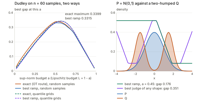
A search over every judge shape on a grid. A chain dynamic programme over judge heights (steps of at most L\,dx between neighbouring grid points, heights within \pm a) finds the best judge of any shape on the grid [-12,12] with 961 points. For N(0,1) against N(1,1): any shape 0.2217, ramp 0.2234 at a=0.30; any shape 0.3426, ramp 0.3427 at a=0.57; any shape 0.2000, ramp 0.2000 at a=0.80. The dynamic programme is a lower bound on a grid; the small deficit at a=0.30 is presumably the rounding of its height limit to the grid of levels, which I did not isolate. Now take P=N(0,1) against Q=\tfrac12N(-1.5,0.5^2)+\tfrac12N(1.5,0.5^2), equal means. The best judge of any shape earns 0.3514 at a=0.45, the best ramp 0.1756: a ratio of 2.001. The optimal judge is high at P’s centre and low at each hump of Q (Figure 3, right); a monotone ramp can serve only one hump. The other distances for this pair are \mathrm{TV}=0.5254, W_1=0.7041 and \mathrm{KL}(P\Vert Q)=1.1584. Widget 1 shows this judge.
7. Kernel judges: MMD
The panel. A kernel k(x,y) is a similarity between outcomes, such as the Gaussian e^{-(x-y)^2/2\sigma^2}. It comes with a space \mathcal H_k of functions built from it (the RKHS of the HSIC page §3: functions f=\sum_i\alpha_ik(z_i,\cdot), each a sum of bumps of the similarity, with \lVert f\rVert^2=\sum_{ij}\alpha_i\alpha_jk(z_i,z_j)). The MMD panel is the unit ball \{f:\lVert f\rVert_{\mathcal H_k}\le1\}. The defining property, “reproducing”, is f(x)=\langle f,k(x,\cdot)\rangle: evaluating f is a dot product.
Closed form. Let \mu_P=\mathbb E_Pk(x,\cdot), the average of the bumps, a point of \mathcal H_k. Then \mathbb E_Pf=\langle f,\mu_P\rangle, so the gap of f is \langle f,\mu_P-\mu_Q\rangle, and by Cauchy–Schwarz the best unit-norm f is the direction of \mu_P-\mu_Q and earns its length:
\mathrm{MMD}(P,Q)=\lVert\mu_P-\mu_Q\rVert_{\mathcal H_k},\qquad \mathrm{MMD}^2=\mathbb E\,k(x,x')+\mathbb E\,k(y,y')-2\,\mathbb E\,k(x,y),
with x,x'\sim P and y,y'\sim Q independent (expand the squared norm using \langle k(x,\cdot),k(x',\cdot)\rangle=k(x,x')). The best judge is the witness w=\mu_P-\mu_Q, normalised: f^*=w/\lVert w\rVert. On samples, w(t)=\tfrac1n\sum_ik(x_i,t)-\tfrac1m\sum_jk(y_j,t): drop a bump at every P sample, subtract a bump at every Q sample.
Four points. X=(-1,0,0.5,2), Y=(0.5,1.5,2,3.5), \sigma=1. The biased estimate (all pairs, diagonal included) is \mathrm{MMD}^2=0.296381, so \mathrm{MMD}=0.544409. The witness at t=-1,0,1,2,3 is 0.3906,\ 0.3199,\ -0.0461,\ -0.2652,\ -0.2989: positive on the left where P has its samples, negative on the right. Three checks: the normalised witness earns 0.544409; 200000 random unit-norm judges in the span of the eight points never exceed 0.543370; and the identity \bar w(X)-\bar w(Y)=\lVert w\rVert^2 holds (0.296381 on both sides). The unbiased estimator, which drops the diagonal terms, gives -0.013221 here: it is centred on the truth and can be negative.
Gaussians. For x-y\sim N(\mu,v) one has \mathbb E\,e^{-(x-y)^2/2\sigma^2}=\dfrac{\sigma}{\sqrt{\sigma^2+v}}\,e^{-\mu^2/(2(\sigma^2+v))}. For N(0,s^2) against N(m,s^2) this gives
\mathrm{MMD}^2=\frac{2\sigma}{\sqrt{\sigma^2+2s^2}}\Big(1-e^{-m^2/(2(\sigma^2+2s^2))}\Big).
At s=\sigma=1, m=1: \tfrac{2}{\sqrt3}(1-e^{-1/6})=0.17727, \mathrm{MMD}=0.4210, identical to a quadrature of (p-q)^\top K(p-q). From 500+500 samples, averaged over 40 draws, the unbiased estimate is 0.1771 (standard error 0.0039) and the biased one 0.1788; a single draw has standard deviation 0.0249. As m grows the value saturates at \sqrt{2\sigma/\sqrt{\sigma^2+2s^2}}=1.0746: MMD at m=0.5,1,2,4,8 is 0.2171,\ 0.4210,\ 0.7496,\ 1.0366,\ 1.0746.
MMD sits inside the Dudley picture. For a bounded kernel with k(x,x)=1, \lvert f(x)\rvert=\lvert\langle f,k(x,\cdot)\rangle\rvert\le\lVert f\rVert, so the unit ball lies in \{\lvert h\rvert\le1\} and \mathrm{MMD}\le2\,\mathrm{TV}. For the Gaussian kernel also \lvert f(x)-f(y)\rvert\le\lVert k(x,\cdot)-k(y,\cdot)\rVert=\sqrt{2-2e^{-d^2/2\sigma^2}}\le d/\sigma, so f has Lipschitz constant at most 1/\sigma, the unit ball lies in (1+1/\sigma) times the Dudley ball, and \mathrm{MMD}\le(1+1/\sigma)\,\gamma_\beta. Numerically, for N(0,1) against N(m,1) at \sigma=1:
| m | 0.25 | 0.5 | 1 | 2 | 4 |
|---|---|---|---|---|---|
| MMD | 0.1094 | 0.2171 | 0.4210 | 0.7496 | 1.0366 |
| 2\,\mathrm{TV} | 0.1990 | 0.3948 | 0.7658 | 1.3654 | 1.9090 |
| (1+1/\sigma)\,\gamma_\beta=2\gamma_\beta | 0.1751 | 0.3486 | 0.6854 | 1.2876 | 2.1367 |
Both inequalities hold in every column (the second is the tighter one for m\le2 and the first for m=4).
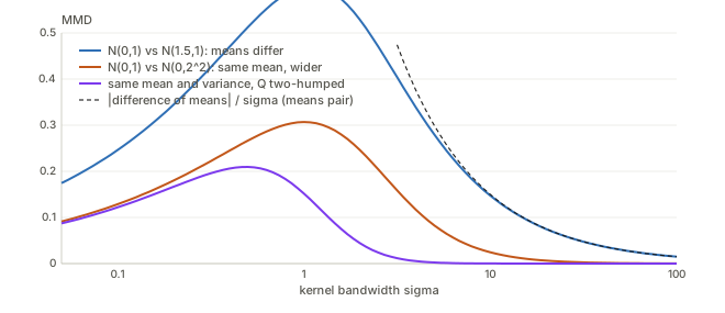
What the bandwidth does. The bandwidth \sigma chooses which judges are in the panel.
- Huge \sigma: only the means. Expanding e^{-u^2/2\sigma^2}\approx1-u^2/2\sigma^2, the constants and the variances cancel and \mathrm{MMD}^2\to(\mu_P-\mu_Q)^2/\sigma^2. For the shifted pair \sigma\cdot\mathrm{MMD} is 0.99984 at \sigma=100; for N(0,1) against N(0,2^2), equal means, it is 0.02596: the kernel has become a linear one and cannot see the width.
- Tiny \sigma: blind. Each sample is only similar to itself; K\to I and the biased estimate tends to the constant 1/n+1/m whatever the samples are. With 40+40 samples and \sigma=0.001 the biased \mathrm{MMD}^2 is 0.04915 for a shifted pair and 0.04894 for two samples of the same law, against 1/40+1/40=0.05000.
- In between. A pair that differs in shape only is found by a mid-range bandwidth: N(0,1.34164^2) against \tfrac12N(-1.2,0.6^2)+\tfrac12N(1.2,0.6^2) (same mean 0 and variance 1.8) has population \mathrm{MMD}^2=0.00756,\ 0.03714,\ 0.02311,\ 0.00019 at \sigma=0.05,\ 0.3,\ 1,\ 3, peaking at 0.04391 near \sigma=0.49.
HSIC. Take P = the joint distribution of pairs (x,y), Q = the product of the marginals, and the product kernel k(x,x')\,l(y,y'). Then \mathrm{MMD}^2=\mathrm{HSIC} (HSIC §5). The witness there says which kinds of pairs are over-represented relative to independence.
8. The big picture
| Distance | Panel of judges | Bounded? | Needs | \delta_0 vs \delta_D (value at D=2) | N(0,1) vs N(m,1) (value at m=1) |
|---|---|---|---|---|---|
| Total variation | 0\le h\le1 | \le1 | nothing | 1 (1.0000) | 2\Phi(m/2)-1 (0.3829) |
| Kolmogorov | half-line indicators \mathbf 1[x\le t] | \le1 | an order (1-D) | 1 (1.0000) | same as TV, single crossing (0.3829) |
| Wasserstein-1 | \lVert h\rVert_L\le1 | no | ground metric d | D (2.0000) | \lvert m\rvert (1.0000) |
| Dudley, sum norm | \lVert h\rVert_L+\lVert h\rVert_\infty\le1 | \le2 | ground metric d | \dfrac{2D}{D+2} (1.0000) | ramp window formula (0.3427) |
| Dudley, max norm | \max(\lVert h\rVert_L,\lVert h\rVert_\infty)\le1 | \le2 | ground metric d | \min(D,2) (2.0000) | not computed |
| MMD, Gaussian kernel | unit ball of \mathcal H_k | \le2 (the shift pair at \sigma=1 tops out at 1.0746) | a kernel (bandwidth \sigma) | \sqrt{2-2e^{-D^2/2\sigma^2}} (1.3150 at \sigma=1) | closed form of §7 (0.4210) |
| KL(P\Vert Q), for contrast | none: a density ratio | no | P\ll Q | \infty | m^2/2 (0.5000) |
The max-norm entry for point masses is a one-line argument (two values in [-1,1] that are D apart under slope \le1 differ by at most \min(2,D)); I did not compute it for Gaussians. The MMD bound of 2 is the reproducing-property argument of §7 (\mathrm{MMD}\le2\,\mathrm{TV}); the point-mass value saturates lower, at \sqrt2.
9. IPMs versus φ-divergences
A \varphi-divergence is D_\varphi(P\Vert Q)=\int q(x)\,\varphi\big(p(x)/q(x)\big)\,dx for a convex \varphi with \varphi(1)=0. KL is \varphi(t)=t\log t, \chi^2 is \varphi(t)=(t-1)^2 and TV is \varphi(t)=\tfrac12\lvert t-1\rvert. In words: at each location, look at the ratio of how much probability P and Q put there, and add up. Two consequences:
- They need overlap. If P puts mass where Q has none, p/q=\infty and KL is infinite. Formally KL needs P\ll Q, “wherever Q has no mass, neither does P”. Embeddings living on thin manifolds are the usual case of non-overlap (the Optimal transport page makes this point for JS, which saturates instead).
- They ignore geometry. Relabelling the outcomes by any one-to-one map leaves every \varphi-divergence unchanged, so \delta_0 against \delta_{0.1} looks like \delta_0 against \delta_{100}.
A picture of the blow-up: narrow the bumps of N(0,s^2) against N(1,s^2) (D=1).
| s | 1 | 0.5 | 0.3 | 0.1 | 0.03 |
|---|---|---|---|---|---|
| \mathrm{KL}=D^2/2s^2 | 0.50 | 2.00 | 5.56 | 50.00 | 555.56 |
| \mathrm{TV} | 0.3829 | 0.6827 | 0.9044 | 1.0000 | 1.0000 |
| W_1 | 1.0000 | 1.0000 | 1.0000 | 1.0000 | 1.0000 |
| Dudley | 0.3427 | 0.4639 | 0.5350 | 0.6196 | 0.6522 |
| MMD (\sigma=1) | 0.4210 | 0.6804 | 0.7975 | 0.8760 | 0.8861 |
KL explodes and TV is stuck at 1; W_1 does not notice the narrowing; Dudley and MMD move smoothly to their point-mass values (2D/(D+2)=0.6667 and \sqrt{2-2e^{-1/2}}=0.8871). Sriperumbudur et al. show that TV is the only non-trivial \varphi-divergence that is also an IPM. That statement is theirs; I did not re-derive it.
10. What the supremum does and does not tell you
Monotone in the panel. If \mathcal F\subseteq\mathcal F' then \gamma_{\mathcal F}\le\gamma_{\mathcal F'}. The Dudley ball is inside the 1-Lipschitz ball and inside the [-1,1] ball: 0.3427\le\min(W_1,2\mathrm{TV})=\min(1,0.7658) for N(0,1) against N(1,1). So a lower bound proved for a small panel holds for every bigger one (for W_1, and for any IPM whose panel contains the Dudley ball), while an upper bound proved for a big panel holds for every smaller one. The converse directions fail: W_1 can be huge while Dudley is at most 2.
To lower-bound a sup, exhibit one judge. Take h(y)=\tfrac12\cos y. Its steepness is \tfrac12 and its height \tfrac12, so \lVert h\rVert_{BL}=1: it is in the Dudley ball. Since \mathbb E\cos y=e^{-\sigma^2/2}\cos f for y\sim N(f,\sigma^2), this judge earns e^{-\sigma^2/2}\lvert\cos f-\cos g\rvert/2 between N(f,\sigma^2) and N(g,\sigma^2). With \sigma=1, f=0:
| g | gap of \tfrac12\cos | true Dudley | fraction found |
|---|---|---|---|
| \pi | 0.6065 | 0.9136 | 66% |
| 2 | 0.4295 | 0.6438 | 67% |
| 1 | 0.1394 | 0.3427 | 41% |
This is the device of Tahir et al.’s Appendix D.1: they use exactly this judge, on the target given the input, to lower-bound the Dudley distance between two target functions in the same feature space (their Theorem A.2), and remark that the result carries over to W_1 by the monotonicity just described. That remark is right. Their statement, though, is that the distance can be made \ge\delta for every \delta>0, which cannot hold for \delta>2 because \gamma_\beta\le2 (§5). The printed proof shows why: its step (29) bounds the gap below by \tfrac12e^{-\sigma^2/2}\int(f^2+g^2)p\,dx, which grows without limit with g, while the quantity above it, \tfrac12e^{-\sigma^2/2}\lvert\int(\cos f-\cos g)\,p\,dx\rvert, is at most e^{-\sigma^2/2}=0.6065 for \sigma=1 since \lvert\cos f-\cos g\rvert\le2. In the code’s one-dimensional analogue, at f=0 and constant g=10 the printed right-hand side is 30.3265; scanning g\in[0,60], the best gap the judge \tfrac12\cos ever earns is 0.6065 (at g=\pi,3\pi,\dots), while the true Dudley distance at g=60 is 1.9304. So as printed the step is false, and the theorem is right only in the reading “as far apart as the metric allows” (for Dudley, arbitrarily close to 2; for W_1 and KL, truly unbounded), which needs a different judge than \tfrac12\cos: a cut-off that separates the two target functions once they are far apart. I checked this only in the one-dimensional Gaussian analogue, not the paper’s joint setting. Their conclusion is a statement about these panels: large distance in Dudley, W_1 or KL need not mean poor transfer, because the panel is not the transfer task.
The panel is not the task. Two ways this bites.
- Far for the panel, identical for the task. P=N(0,I) and Q = P shifted by 3 along coordinate 1 in \mathbb R^2 are at W_1=3, yet every function of coordinate 2 alone has the same average under both (the gap of \tanh z_2 is 0.0000). A downstream head that reads only coordinate 2 does not care.
- Close for the panel, different for the task. Let P=\delta_0 and Q=(1-\varepsilon)\delta_0+\varepsilon\delta_R, a rare far outlier, with \varepsilon=0.01 and R=1000. Then \mathrm{TV}=0.01 and Dudley =\varepsilon\cdot2R/(R+2)=0.01996, while W_1=\varepsilon R=10 and the task f(x)=x changes by 10. A bounded panel cannot register an unbounded task.
Bounded panels saturate. Dudley cannot exceed 2, MMD is capped by its bandwidth, TV by 1. “Arbitrarily far” for these metrics can only mean “as far as the metric allows”. At m=8 the Dudley distance is 1.4688, not close to 2, though the two Gaussians barely overlap.
11. Where it shows up
- WGAN (Arjovsky, Chintala & Bottou 2017): the critic is the 1-Lipschitz judge of §4, and training pushes the generator to shrink its gap. The critic you train is the best judge, so it is inspectable.
- Two-sample tests and generative modelling with MMD (Gretton et al. 2012; MMD-GAN): the witness of §7 is the test’s explanation. The permutation test in widget 3 is the same recipe as the HSIC test.
- Domain alignment with MMD: see the MICCAI 2026 domain-adaptation notes.
- HSIC and CKA: MMD between the joint and the product of marginals (HSIC).
- Theory that must not depend on the panel: Tahir et al. above; lower bounds via one judge, carried to larger panels by monotonicity.
Questions and doubts
- Ramp optimality beyond a symmetric hump. §5.2’s layer argument needs F-G to be a single hump symmetric about its centre. For a single asymmetric hump the bound \int\min(2a,L\lvert I_t\rvert)dt may not be reached by one window, and I have not checked whether the ramp still wins. Gaussians of different widths, the natural next case, have a F-G that changes sign, so §5’s formulas do not cover them at all.
- Dudley depends on the units. The sum norm builds in a length scale of about 1 (§5.4): Dudley/W_1 for small shifts is 0.2278 for s=2 and 0.9683 for s=0.01. If the embedding is rescaled by ten, the Dudley distance changes non-trivially. Which normalisation of an embedding makes “\lVert h\rVert_{BL}\le1” meaningful, and does a claim like “Dudley distance \ge\delta” survive a change of units?
- Sum norm versus max norm. The max-norm value is computed here only for point masses (\min(D,2)). For Gaussians it should be larger than the sum-norm value (the ball is bigger), by how much I did not compute.
- The dynamic programme and the sample ramp search are lower bounds. Only the truncated-cost transport route is exact on samples, and it needs equal-size uniform samples. I verified duality numerically (the Hungarian potentials give a 1-Lipschitz judge that earns W_1), but that is a check on one pair of samples, not a proof.
- High dimensions. Everything numerical here is one-dimensional. In \mathbb R^d the optimal transport cost of samples is known to converge slowly (rate n^{-1/d}) while MMD converges at n^{-1/2}. I recall this from Sriperumbudur et al.’s follow-up work and did not check it here, but it bears on any use of W_1 between embedding clouds.
- Which panel for a downstream task? §10’s two examples say a panel should contain the task’s functions. For a fine-tuning head, the functions of the embedding it can compute form a panel. Is the IPM over that panel computable, and how does it relate to transfer performance? Tahir et al. suggest, in their setting, that feature-space overlap, not a distributional distance, is what matters.
- Can Theorem A.2 be repaired? §10 argues the statement is right only up to the ceiling of 2 and that step (29) of its proof fails. A repair needs a judge that is a Lipschitz cut-off around f, and a bound on the mass of p_g that falls outside it. I have not written that proof, and I have not checked the KL half of the theorem (KL is unbounded, so no ceiling problem arises there).
- Citations from memory. Müller (1997), Dudley (2002), Gretton et al. (2012) and the statement that Dudley metrises weak convergence are recalled, not re-checked. The claim that TV is the only common member of the two families is quoted from the abstract of Sriperumbudur et al.
Takeaways
- An IPM is the gap of the best judge from a panel: \gamma_{\mathcal F}=\sup_{h\in\mathcal F}\lvert\mathbb E_Ph-\mathbb E_Qh\rvert. The panel is the distance: [0,1]-valued gives TV, 1-Lipschitz gives W_1, height plus steepness at most 1 gives Dudley, the unit ball of a kernel gives MMD.
- In one dimension a ramp judge earns L\times the area between the two CDFs over its sloping window. W_1 is the whole area, and Dudley is the best window under a height budget. For N(0,1) against N(1,1): \mathrm{TV}=0.3829, Dudley =0.3427, W_1=1, \mathrm{KL}=0.5, \mathrm{MMD}=0.4210.
- Two point masses give closed forms: \mathrm{TV}=1, W_1=D, Dudley =2D/(D+2), \mathrm{KL}=\infty. Bounded panels saturate (TV at 1, Dudley at 2, MMD at \sqrt2 for the Gaussian kernel and point masses); W_1 and KL do not.
- MMD has a closed form, \mathbb E k(x,x')+\mathbb E k(y,y')-2\mathbb E k(x,y), and a witness function that shows where P and Q differ. The bandwidth is a choice of panel: huge sees only means, tiny sees nothing.
- A bigger panel gives a bigger sup, so lower bounds transfer upward. To lower-bound a sup, exhibit one judge.
- The sup is over your panel, not the downstream task’s: a large IPM does not imply a hard task, and a small bounded IPM does not imply a benign one.