Not All Models Are Equal: Predicting Model Transferability in a Self-challenging Fisher Space
Links
- arXiv:2207.03036 — preprint; ECCV 2022. Code at TencentARC/SFDA.
- The measures it builds on and competes with: Nguyen 2020 — LEEP, You 2021 — LogME, Bao 2019 — H-score.
- Claßen 2026 — TE robustness — reports SFDA producing NaNs on medical targets, “due to all source models being assigned the same score”.
- LDA / Fisher discriminant and principal angles — the background this leans on.
- Achille 2019 — task reachability — models fine-tuning directly, as noisy gradient descent from the source weights. SFDA’s self-challenging step is the one heuristic among these scores meant to imitate those dynamics. The linked section compares every score here with the paper’s static and dynamic factors.
- Runnable
code — ConfMix as a difficulty amplifier, the D'=\min(D,C-1) collapse on binary
targets, the three incompatible statements of \lambda, and what \lambda=1 costs.
make verifyruns it.
In one paragraph
Every earlier measure scores a pre-trained model by its static features. SFDA’s argument is that fine-tuning does not leave features static — it separates classes and it learns hard examples late — so a good proxy should imitate both. It does this in two stages. First, Reg-FDA projects the frozen features into a regularised Fisher space where classes are more separable, and an LDA classifier there gives a per-sample confidence. Second, ConfMix perturbs each sample toward the mean of the other classes by exactly its current difficulty, and Reg-FDA is run again on the harder problem. The score is the average log-likelihood after that second pass. It works well on the paper’s 11 benchmarks and, as a bonus, projects every model into a common C-1 dimensional space, which makes ensemble selection possible. It is also the one measure in this section that both medical benchmarks report failing outright, and the reasons are visible in the construction.
The spine of the argument
- Static-feature metrics cannot see the fine-tuning dynamics. Imitate two of them instead.
- Class separability: project into a Fisher space (Reg-FDA), classify by LDA, take the log-likelihood.
- Hard examples: make the problem harder in proportion to existing difficulty (ConfMix), then redo step 2. Models that still separate are the ones that fine-tune well.
- Free consequence: all models land in the same C-1 dimensions, so they become comparable and ensembles can be scored.
Setup and notation
| Symbol | Meaning |
|---|---|
| \hat x = \theta_m(x)\in\mathbb{R}^D | the static feature from pre-trained model m |
| C, N_c | number of target classes, and samples in class c |
| S_B, S_W | between- and within-class scatter |
| \tilde S_W=(1-\lambda)S_W+\lambda I | the regularised within-class scatter |
| U\in\mathbb{R}^{D\times D'} | the Fisher projection, \bar x = U^\top\hat x |
| D'=\min\{D,\,C-1\} | the Fisher space’s dimension |
| p_n | confidence of the LDA classifier on sample n |
| \tilde x_n | the ConfMix-perturbed feature |
Stage 1 — Regularised FDA
U=\arg\max_U \frac{d_B(U)}{d_W(U)}=\frac{\lvert U^\top S_BU\rvert} {\lvert U^\top[(1-\lambda)S_W+\lambda I]U\rvert} \tag{2}
which is ordinary Fisher discriminant analysis with a shrinkage term, solved as a generalised eigenproblem S_Bu_k=v_k\tilde S_Wu_k (Eq. 4) — no gradient descent, which is the efficiency claim. Classification in that space is LDA with \Sigma_c=I assumed:
\delta_c(\hat x_n)=\hat x_n^\top UU^\top\mu_c-\tfrac12\mu_c^\top UU^\top\mu_c+\log q_c, \qquad p(y_n\mid\hat x_n)=\frac{e^{\delta_{y_n}}}{\sum_c e^{\delta_c}} \tag{5, 6}
and the score is T_m=\sum_n\log p(y_n\mid x_n) (Eq. 1).
One structural consequence worth pulling out. \operatorname{rank}(S_B)\le C-1 always, so D'=\min\{D,C-1\}. The paper presents this as a feature — every model projects to the same C-1 dimensions regardless of its native width, which is what makes ensemble comparison possible. But it also means a binary target gives a one-dimensional Fisher space: every model is scored through a single direction. That is exactly the setting in which Claßen et al. report SFDA assigning every source the same score, and then NaN when a rank correlation is taken.
| classes C | 2 | 5 | 10 | 100 |
|---|---|---|---|---|
| Fisher dimensions D' | 1 | 4 | 9 | 99 |
Stage 2 — ConfMix, the idea worth keeping
\tilde x_n=p_n\hat x_n+(1-p_n)\,\mu_{c\neq y_n} \tag{7}
Each sample is moved toward the mean of the classes it does not belong to, by exactly (1-p_n) — its own current difficulty. A confidently classified point barely moves; an ambiguous one is dragged most of the way across. Reg-FDA is then re-run on \{\tilde x_n\}, and the final score comes from that second pass.
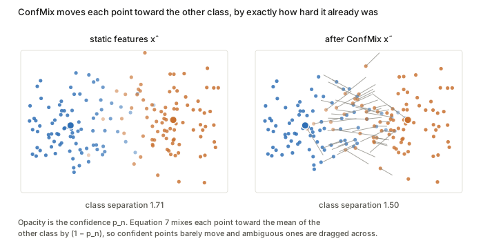
This is a genuinely nice mechanism and the paper’s best idea. It is a difficulty amplifier: it does not add uniform noise, it widens exactly the gap between models that handle ambiguous samples and models that do not. Since fine-tuning learns easy examples early and hard ones late (their Fig. 3d), amplifying difficulty is a reasonable proxy for late-stage fine-tuning behaviour. Self-supervised augmentation used as a measurement instrument rather than a training one is an idea that transfers.
The regularisation strength is specified three incompatible ways
This is the part that needs stating plainly, because it is not a typo in one place.
| where | formula |
|---|---|
| Eq. 3, main text | \lambda=\exp^{-a\sigma(S_W)} |
| text immediately after Eq. 3 | refers to “\sigma(S_B) in Eqn. (3)” |
| Algorithm 1, line 11 (Appendix A.2) | \lambda=1/(1+\exp^{-a\sigma(S_B)}), with a=4 |
The first decreases in its argument; the third increases, in a different matrix. These are not variants of one formula. And at the stated a=4, on realistically sized scatter matrices, the two written forms saturate at opposite ends:
| setting | \sigma(S_W) | \sigma(S_B) | Eq. 3 | Alg. 1 |
|---|---|---|---|---|
| small, low-dim | 2858 | 12559 | 9.9e−305 | 1.0000 |
| typical CNN | 4471 | 122092 | 9.9e−305 | 1.0000 |
| binary medical | 926 | 16427 | 9.9e−305 | 1.0000 |
| wide backbone | 3681 | 107544 | 9.9e−305 | 1.0000 |
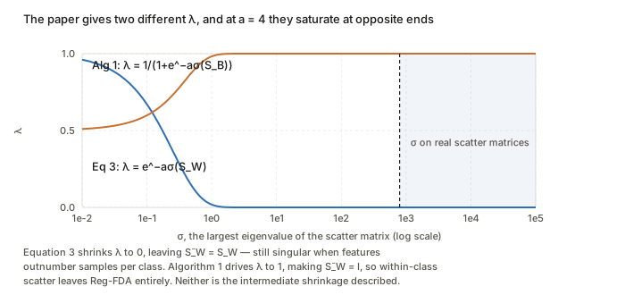
Both endpoints are bad, in different ways:
- \lambda\to0 leaves \tilde S_W=S_W, so a singular S_W stays singular. Juodelyte et al. identify exactly this: when the feature dimension exceeds the samples per class, S_W is rank-deficient and the projection can collapse a class onto a point. The shrinkage term exists to prevent that, and Eq. 3 switches it off precisely when it is needed.
- \lambda\to1 makes \tilde S_W=I exactly, so Eq. 2 becomes \lvert U^\top S_BU\rvert/\lvert U^\top U\rvert and U is just the eigenbasis of S_B — the within-class scatter has left the method entirely. Verified: the \lambda=1 subspace and S_B’s eigenbasis have principal-angle cosines [1,1,1,1].
How much the second costs depends on how anisotropic the within-class scatter is — which is the case Reg-FDA exists to handle:
| anisotropy | 1 | 5 | 25 |
|---|---|---|---|
| nearest-centroid accuracy, Reg-FDA | 1.000 | 0.965 | 0.606 |
| nearest-centroid accuracy, \lambda=1 | 1.000 | 0.877 | 0.385 |
With isotropic noise \lambda hardly matters. As the scatter becomes anisotropic the subspaces diverge and accuracy in the \lambda=1 space falls away. Their own ablation (Table 3, variant 3) reports that a fixed \lambda=0.5 is worse than the adaptive rule — but if the adaptive rule is in fact saturating at 1, what that ablation compares is 0.5 against 1, not against adaptivity.
Ensembles, which is the other contribution
Because D'=C-1 is the same for every model, features from different backbones can be stacked into F^{\mathrm{ens}}\in\mathbb{R}^{M\times D'} and a complementarity score computed by ablation on the nuclear norm:
T^{\mathrm{com}}_m=\lVert F^{\mathrm{ens}}\rVert_*-\lVert F^{\mathrm{ens}}\odot1_m\rVert_*, \qquad T^{\mathrm{ens}}_m=rT^{\mathrm{SFDA}}_m+(1-r)T^{\mathrm{com}}_m \tag{8, 9}
with r=0.5. The nuclear norm is a convex relaxation of rank, so T^{\mathrm{com}}_m measures how much model m raises the rank of the ensemble — how much it adds that the others do not. This is the first measure in the section to score a set rather than a single model, and the homogenisation that makes it possible is a real benefit of the Fisher projection.
Results, briefly
Weighted Kendall’s \tau_w against fine-tuned accuracy across 11 targets and 11 supervised CNNs: SFDA is best on 8 of 11, and the gains over NLEEP are large where they occur (+0.327 on Flowers, +0.191 on Food, +0.160 on Pets). Against NLEEP it is also 22.5× faster in wall-clock — 91.9s versus 253.8s on Aircraft, and far more at the extremes (75.0s versus 678.8s on VOC). It is slower than LEEP and LogME, which the paper concedes while arguing those are less stable.
Questions and doubts
- The \lambda specification is the central problem. Three incompatible statements, and at the stated a=4 both written forms saturate. Whatever the released code does, the paper as written does not describe a method that performs intermediate shrinkage, and the adaptivity claim — the subject of an ablation — cannot be checked from the text.
- D'=C-1 collapses binary targets to one dimension. Presented as a feature for ensembles, it is a liability for the many two-class medical tasks, and it is the most likely proximate cause of the reported ties and NaNs.
- The self-challenging stage runs exactly once. ConfMix is applied, Reg-FDA repeated, done. Nothing motivates one round rather than a schedule, and if the analogy to late-stage fine-tuning is taken seriously a schedule is the natural object.
- \Sigma_c=I in the Fisher space is assumed “for simplicity” (Eq. 5). That is the same isotropy assumption whose failure makes \lambda matter, imposed one stage later without comment.
- Classification only, as the conclusion concedes: no regression, and no out-of-distribution analysis — the two axes LogME and Chaves et al. respectively cover.
- The ensemble score is barely evaluated. r=0.5 is “empirical”, the nuclear-norm ablation is O(M) refactorisations, and the comparison is relegated to an appendix.
Takeaways
- ConfMix is the transferable idea: perturb each sample by its own difficulty, and you have an instrument that magnifies differences between models exactly where those differences matter. It is a measurement use of augmentation, and it is not specific to transferability.
- Projecting to C-1 dimensions homogenises models, which is what unlocks ensemble scoring — genuinely novel in this section — and simultaneously what breaks the method on binary targets. One design decision, both consequences.
- Read Eq. 3 against Algorithm 1 before implementing. They disagree about the formula, the matrix, and the direction, and at a=4 both saturate. This is the concrete reason to reach for the released code rather than the paper.
- Against the rest of the section, SFDA is the only measure that tries to model fine-tuning as a process rather than scoring a static representation. That ambition is right, and the failure reports in the medical benchmarks are about the implementation of the regulariser rather than about the ambition.