Path-Decoupled Hyperbolic Flow Matching for Few-Shot Adaptation
Links
- arXiv:2602.20479 —
preprint.
make fetchpulls the PDF from here. - Runnable
code — the Lorentz primitives of Section 3.1, verified to
machine precision, plus a quantitative test of the paper’s geometric
claim.
make verifyruns it.
In one paragraph
CLIP few-shot adaptation usually applies a one-step correction: an adapter or prompt shifts visual features toward text prototypes in a single forward pass. FMA instead treats it as continuous transport — learn a velocity field carrying image features to their class’s text region and integrate, giving multi-step iterative rectification. Li et al. argue those Euclidean paths collide, because flat geometry has only polynomial volume growth and there is not enough room. Their fix reformulates the transport on the Lorentz manifold, whose exponential volume growth gives space to separate: text prototypes are anchored near the origin as semantic roots, images pushed to the boundary as leaves, and the flow is supervised step-wise with a contrastive “guardrail” on each intermediate state. A diameter-based stopping rule halts transport before features crowd into the origin.
The spine of the argument
- Euclidean flow matching suffers path entanglement — trajectories from different classes intersect and get diverted by dense neighbours.
- Hyperbolic space has exponentially more room at radius R, so put the flow there.
- Centripetal alignment (§3.2) imposes a text-root / image-leaf hierarchy via an entailment cone loss, turning arbitrary transport into ordered inward flow.
- Path-decoupled objective (§3.3) supervises the predicted next state rather than the velocity, which allows a contrastive term on intermediate states — the “semantic guardrail”.
- Diameter-based stopping (§3.4) terminates before the crowded origin.
Setup and notation
| Symbol | Meaning |
|---|---|
| \mathbb{L}^{n,\kappa} | Lorentz model, learnable curvature -\kappa (\kappa initialised to 1) |
| \langle x,y\rangle_L | -x_0y_0 + \langle\tilde x,\tilde y\rangle_E; points satisfy \langle x,x\rangle_L = -1/\kappa |
| x_0, x_1 | source (image feature, leaf) and target (text prototype, root) |
| \alpha_{txt} < \alpha_{img} | learnable norm scalars placing text near origin, images near boundary |
| \omega(x_1) | entailment cone half-aperture, \arcsin(2H/\lVert x_1\rVert_L), H = 0.1 |
| \delta | flow step size |
| \Pi_{T_zL} | orthogonal projection onto the tangent space at z |
| d_{txt} | semantic diameter, \max_{i,j} d_L(x_1^i, x_1^j) |
| \phi(N) | stopping scale, 0.5\log_{10}(N) for N classes |
| \lambda | weight on the inter-class decoupling loss (0.1) |
The primitives (§3.1)
d_L(x,y) = \tfrac{1}{\sqrt\kappa}\operatorname{arcosh}(-\kappa\langle x,y\rangle_L), \qquad \Pi_{T_zL}(x) = x + \kappa\langle z,x\rangle_L\, z
\log^\kappa_z(x) = \frac{\operatorname{arccosh}(-\kappa\langle z,x\rangle_L)}{\sqrt{\langle z,x\rangle_L^2 - 1/\kappa^2}}\,\Pi_{T_zL}(x), \qquad \exp^\kappa_z(u) = \cosh(\lVert u\rVert)z + \sinh(\lVert u\rVert)\tfrac{u}{\lVert u\rVert}
code/lorentz.py checks all of these to machine
precision, including that their geodesic x_t =
\exp_{x_0}(t\log_{x_0}(x_1)) is constant speed:
d_L(x_0,x_t)/d_L(x_0,x_1) = t
exactly.
Component 1 — centripetal hyperbolic alignment (§3.2)
Two learnable scalars \alpha_{txt} < \alpha_{img} rescale Euclidean feature norms before the \exp_0 projection, placing text near the origin and images near the boundary. Blunt, but it establishes the hierarchy.
The entailment cone loss, inherited from MERU (Desai et al.):
\mathcal{L}_{entail} = \max\big(0,\; \pi - \angle 0x_1x_0 - \omega(x_1)\big), \qquad \omega(x_1) = \arcsin\!\big(2H/\lVert x_1\rVert_L\big)
The exterior angle at the prototype, between its radial axis and the direction to the image, must lie inside a cone of half-aperture \omega. The crucial detail is that \omega shrinks as \lVert x_1\rVert grows — prototypes near the origin get wide cones and can entail many leaves, distant points get narrow ones. That is what makes the hierarchy self-consistent rather than an arbitrary radial ordering. A hyperbolic contrastive loss (ordinary InfoNCE with -d_L/\tau replacing cosine) supplies class discrimination.
Component 2 — path-decoupled flows (§3.3)
Ground truth is the geodesic from each image to its own prototype, which is what makes the conditional paths independent across classes. The network predicts an ambient vector, projected to the tangent space and pushed back to the manifold:
v_t = \Pi_{T_{x_t}L}\big(F_\theta(x_t,t)\big), \qquad \hat x_{t+\delta} = \exp^\kappa_{x_t}(\delta v_t)
Then two losses, both on the predicted next state:
\mathcal{L}_{step} = \big\lVert d_L(\hat x_{t+\delta}, x_{t+\delta})\big\rVert^2, \qquad \mathcal{L}_{icd} = -\log\frac{\exp(-d_L(\hat x_{t+\delta}, x_1^c)/\tau)}{\sum_k \exp(-d_L(\hat x_{t+\delta}, x_1^k)/\tau)}
This is the substantive departure from flow matching. Standard Riemannian FM regresses the velocity against a conditional target. Supervising the resulting state in geodesic distance is what allows a contrastive term to be attached to an actual manifold point — impossible with velocity supervision. Their Table 10 shows the two design choices interact rather than being independently good:
| velocity supervision | step-wise | gain | |
|---|---|---|---|
| FMA (Euclidean) | 77.7 | 77.8 | +0.1 |
| HFM (hyperbolic) | 78.8 | 79.8 | +1.0 |
Worth naming plainly: with fixed \delta and state supervision this is closer to a learned discrete transport map or consistency model than to flow matching. No marginal-preserving property is claimed or used. “Flow matching” is doing loose duty in the title.
Component 3 — diameter-based stopping (§3.4), and why it is load-bearing
\min_c d_L(\hat x_{t^*}, x_1^c) \le \phi(N)\cdot d_{txt}, \qquad \hat y = \arg\min_c \sum_{t\le t^*} d_L(\hat x_t, x_1^c)
Presented as an efficiency measure. It is more than that, and
code/lorentz.py shows why. Taking two class trajectories
with sources at hyperbolic radius 4 and targets near the origin, holding
the angular separation fixed so the geometries are compared like for
like:
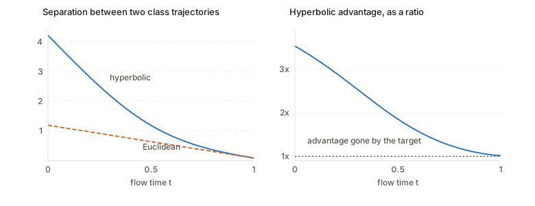
So the stopping rule is structurally required, not an add-on: the geometry stops helping exactly where the flow is heading. The paper presents it as a third independent contribution; it is better understood as a necessary patch for a limitation of the first two. That reframing makes the design coherent rather than arbitrary.
The capacity argument itself does check out — in a 2-D slice, a sphere of radius R holds 2\pi\sinh R points at unit spacing versus 2\pi R, which at R = 8 is 186× more room. The issue is not whether hyperbolic space is roomy; it is that the roominess is at the boundary, and the target is not.
Results
Ablation on difficult benchmarks, 16-shot: baseline 76.1 → +CHA 77.7 → +PO 79.2 → +DS 79.8.
The control experiment I would have demanded, and they ran it (Table 9): FMA* applies HFM’s exact objectives in Euclidean space.
| avg | |
|---|---|
| FMA (Euclidean, velocity) | 77.7 |
| FMA* (Euclidean, HFM’s objectives) | 77.9 |
| HFM (hyperbolic) | 79.8 |
Objectives alone: +0.2. Geometry: +1.9. Clean attribution, and it supports their claim.
It is also plug-and-play across PEFT methods, with the largest gains on the weakest baselines (CoCoOp +8.2, CLIP-Adapter +8.7, CLIP-LoRA +3.7) — consistent with “it fixes entanglement”, since weaker adapters leave more entanglement to fix. Overhead is modest: +0.06M parameters, +27% train step, +19% inference.
Questions and doubts
- Direct evidence for the headline claim is thin. Their own Trajectory Entanglement Rate moves 30.2% → 27.8%, just 2.4 points against a 2.1-point accuracy gain. TER is introduced only in the appendix and is their own proxy. The FMA* control is good; the entanglement story itself is supported mostly indirectly.
- “Isolated geodesic corridors” is an overstatement. The figure above shows the corridors merging as the target is approached. They are real at the boundary and fictional near the origin.
- \phi(N) = 0.5\log_{10}(N) is unmotivated and odd. For N \ge 100 it exceeds 1, so the stopping radius is larger than the entire semantic diameter; for ImageNet (N = 1000, \phi = 1.5) the flow should terminate almost immediately. No ablation on this function, and it is the one hyperparameter doing task-dependent work.
- Most of the gain is the prior, not the flow. Their Table 6 shows the entailment loss alone reaching 79.0 of the final 79.8. The centripetal hierarchy — imposed by two hand-set scalars — carries most of the benefit, with the learned transport adding under a point.
- \kappa is learnable, initialised at 1.0, and never reported. What it converges to is the most direct test of whether hyperbolicity is being used at all; if \kappa \to 0 the space flattens and the thesis collapses. Its absence is conspicuous.
- No theory, despite a thoroughly geometric framing. Every claim is empirical.
Takeaways
- The geometric intuition is sound and quantifiable: exponential volume growth really does give exponentially more room to separate trajectories, and the capacity calculation is a one-liner worth carrying.
- That room is at the boundary. Any method transporting into a crowded region recovers the Euclidean situation near its target, which is a general lesson for hyperbolic transport methods, not a quirk of this paper.
- Supervising the predicted state instead of the velocity is the genuinely transferable modelling idea, and it is what makes an intermediate-state contrastive term possible.
- Running the Euclidean control with matched objectives is the right way to attribute a gain to geometry, and more papers making geometric claims should do it.