Large Scale Structure of Neural Network Loss Landscapes

Stanislav Fort (Google Research), Stanislaw Jastrzebski (NYU) · NeurIPS · 2019

In one paragraph

Two networks trained from different random starts have a high loss wall on the straight line between their weights, yet a curve between them with no wall exists. The paper proposes a picture that makes both facts unsurprising: the set of good weight vectors is a union of huge flat pieces, wedges, each stretching far in n directions and thin in the other D-n, with n only slightly below the full dimension D. Any two wedges intersect, so you can go from one to the other along the intersection, while the straight line between two points on different wedges leaves both. The paper does three things with the picture. It builds the corresponding toy loss and shows the toy reproduces known behaviour (low-dimensional training, connectors between pairs). It predicts and finds low-loss connectors between many optima at once (m-connectors). And it explains when averaging weights (SWA) works and when it fails.

The spine of the argument

Modes are connected by curves, not lines. Linear interpolation hits a wall but a curved connector exists (Draxler et al. 2018, Garipov et al. 2018).
In high dimension, “walls” and “valleys” from 2-D pictures mislead. Model the low-loss set as a union of n-dimensional wedges in D dimensions, with s=D-n\ll D short directions.
Consequences, all checked against the toy: any two wedges intersect; the straight line between points on different wedges leaves them; a hyperplane of dimension d reaches a wedge iff d\ge D-n (the intrinsic dimension); a path switching wedges has deviations from the line aligned within each half and orthogonal across halves.
Predicted and then found: tunnels connect not only pairs but m+1 optima (m-connectors).
Regularisers (learning rate, L2, dropout) widen the tunnel the optimiser travels in; larger batch narrows it.
SWA averages snapshots, which only lands in the low-loss set if the snapshots share a wedge.

Setup and notation

Symbol	Meaning
D	number of weights (dimension of weight space)
n, s=D-n	long (free) dimensions of a wedge, and its short (thin) directions
n-wedge	a cuboid long along n coordinate axes, thin along the rest; one for every choice of n axes
L_{\rm toy}(P)	surrogate loss: Euclidean distance from P to the nearest wedge
optimum, mode	a point where L_{\rm toy}=0 (on a wedge); in a real network, a trained solution
connector, tunnel	a path between two optima along which the loss stays low
m-connector	a low-loss m-dimensional surface through m+1 optima
d_{\rm int}	intrinsic dimension: smallest random-hyperplane dimension in which training still works (Li et al. 2018)
SWA	stochastic weight averaging: average the weights of several snapshots

The toy model

The loss. To get the distance to the nearest axis-aligned wedge, sort |P_1|,\dots,|P_D|, take the s=D-n smallest, and

L_{\rm toy}(P)=\sqrt{\textstyle\sum_{i\in\text{the }s\text{ smallest}}P_i^{\,2}} .

A point has zero loss exactly when at least s of its coordinates are zero (then it lies on the wedge whose short directions are those coordinates). Gradient descent on \tfrac12L_{\rm toy}^2 updates only the currently smallest s coordinates, P_i\leftarrow P_i-\eta P_i, shrinking them geometrically to zero and leaving the other n coordinates where they were. In the code, a random start therefore lands on a random wedge and keeps its norm (\lVert A\rVert=9.65 for D=100): “the radius stays and the optimiser moves along a tunnel”.

Why the straight line leaves the wedges. Let A have zero set Z_A and B have Z_B, both of size s. At the midpoint \tfrac12(A+B) the coordinates in Z_A\cap Z_B are zero, those in Z_A\setminus Z_B equal B_i/2, those in Z_B\setminus Z_A equal A_i/2, and the rest are (A_i+B_i)/2. So the number of zero coordinates is |Z_A\cap Z_B|<s unless the two share a wedge, and the loss is positive. (My derivation; the paper states the conclusion.) Two random wedges share about s^2/D short directions, i.e. almost none.

Why the intersection exists. The intersection of two wedges has zeros in Z_A\cup Z_B, so it has about 2s short directions. It is a smaller wedge but nonempty: it contains every point whose coordinates on Z_A\cup Z_B are zero. Moving from A to B along it is the connector of Figure 1.

The intrinsic dimension. A random d-dimensional hyperplane meets an n-dimensional set in D dimensions generically when d+n\ge D, i.e. d\ge D-n=s. So in the toy d_{\rm lim}=D-n, which the paper identifies with the intrinsic dimension d_{\rm int} of Li et al. (2018).

Check 1: two optima, the straight line, and the midpoint

(D=100, n=90, s=10.) Two random starts optimised to zero loss have |Z_A|=|Z_B|=10 zero coordinates and share 0 of them (a random pair would share about s^2/D=1). The midpoint has 0 zero coordinates, against the 10 a wedge point needs. Loss on the straight line: max 0.287 (at t=0.14); midpoint 0.148. Compare \lVert A\rVert=9.65: in the toy the wedge thickness is zero, so any positive loss is a wall, but its size is small next to the norm.

Check 2: the tunnel algorithm of Section 4.2

The algorithm: cut the line into segments; at each point put a (D-1)-dimensional hyperplane normal to the line; minimise the loss inside it, starting from the line; join the optimised points. The toy version (100 segments) gives loss \le10^{-119} at all 101 optimised points. The polyline joining them has max loss 0.071 (straight line: 0.287), the small excess coming from consecutive points lying on different wedges.

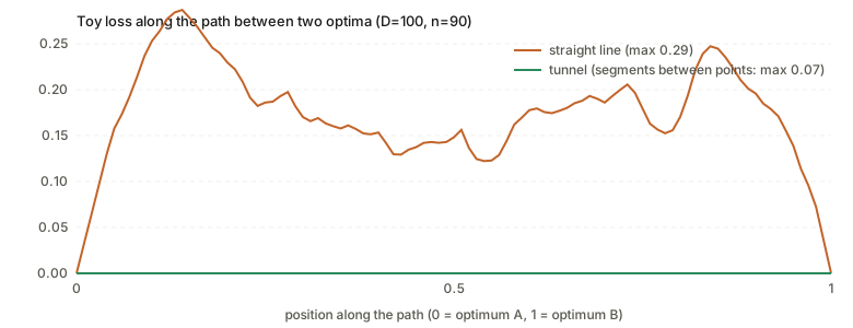
A plot of the toy loss against position along the path from optimum A to optimum B. The straight line is a curve that rises to about 0.29 near the start, dips to about 0.12 near the middle and rises again to about 0.25 before returning to zero. The tunnel is flat at zero.

One random pair. The straight line (orange) has a wall along its whole length; the tunnel (green) sits on the floor. The small bumps in the straight line are real: the loss is a sorted-coordinate function, so its derivative jumps where the ordering of coordinates changes.

The alignment claim (their Figure 3, middle). The deviation of each tunnel point from the line, as a vector, is \delta_k=p_k-\big((1-t_k)A+t_kB\big). Cosines between deviations: within the first half 0.24, within the second half 0.28, across halves +0.01. So the deviations are positively aligned inside each half and orthogonal across, as the paper reports for real networks. (Aligned but not parallel: 0.24–0.28, not 1.)

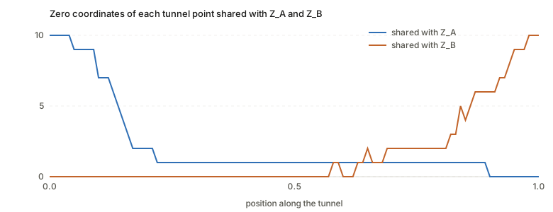
What the tunnel does (not stated in the paper). Tracking which short directions each tunnel point shares with Z_A and Z_B, at t=0,0.1,\dots,1:

	0	.1	.2	.3	.4	.5	.6	.7	.8	.9	1
shared with Z_A	10	7	2	1	1	1	1	1	1	0	0
shared with Z_B	0	0	0	0	0	0	0	2	2	6	10

Every point has exactly 10 zero coordinates, so each sits on one wedge. But through the middle of the path the points share 0–1 of them with either end: the tunnel does not hop from wedge A straight to wedge B. It travels over a series of intermediate wedges, each close to the previous one.

Two curves of shared zero coordinates along the tunnel. The count shared with optimum A falls from ten to one by a position of 0.2 and stays at one until 0.9. The count shared with optimum B stays near zero until about 0.65 and rises to ten at the end.

Check 3: random hyperplanes and the intrinsic dimension

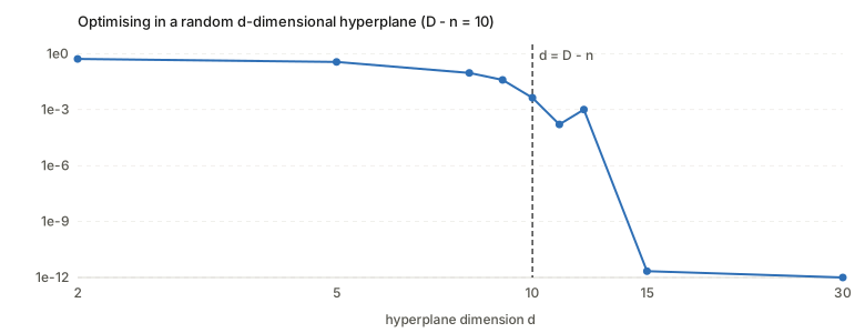
Start at a random point, optimise inside a random d-dimensional hyperplane; median final loss over 5 draws (D-n=10):

d	2	5	8	9	10	11	12	15	30
loss	0.52	0.36	0.094	0.039	4.4e−3	1.6e−4	1.0e−3	2e−12	4e−46

The loss falls steeply across d\approx D-n=10 and is numerically zero by 15. The edge is blurred rather than sharp because 3000 gradient steps cannot finish convergence when the hyperplane only just reaches a wedge.

Median final toy loss against random hyperplane dimension on a log scale. It stays between 0.5 and 0.04 below dimension 10, drops to about 4e-3 at 10, and reaches 1e-12 at 15.

Check 4: m-connectors

Take m+1 optima, pick random points of their convex hull (average loss before: 0.11–0.16 depending on m), project the gradient to a hyperplane of dimension D-m orthogonal to the hull, optimise from the point. Loss after: 0 (below 10^{-100}) for m=1,2,4,6,10. The dimension count explains it: a hyperplane of dimension D-m meets an n-dimensional set when (D-m)+n\ge D, i.e. m\le n=90, far above the 10 the paper tests.

Check 5: averaging, and the SWA prediction

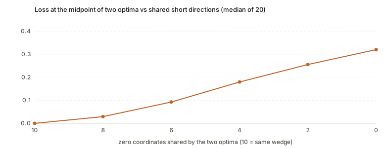
Two optima that share j of their 10 zero coordinates, with other coordinates random: the loss of their average is \sqrt{} of the sum of the 10 smallest squares of the averaged vector, so each short direction not shared contributes a half-sized nonzero coordinate. Median over 20 draws:

shared zero coordinates	10	8	6	4	2	0
loss at the midpoint	0.000	0.029	0.093	0.180	0.255	0.320

So averaging is free inside one wedge and costs more the less the two optima share. This is the model’s reading of the SWA figure: at low learning rate the snapshots stay on one wedge and their mean is good; at high learning rate they move between wedges and the mean falls out.

The loss of the midpoint of two optima against the number of shared zero coordinates: 0 when ten are shared, rising to 0.32 when none are shared.

The experiments on real networks

Section	What they did	What they found
4.2	Build tunnels between pairs of CNN optima (CIFAR-10, Fashion-MNIST) by the algorithm above	low-loss connectors; deviations aligned within each half, orthogonal across halves (Fig. 3); predicted labels change linearly up to the midpoint, then stay constant; short directions at the ends \approx300, close to the CNN’s intrinsic dimension
4.3	Extend to m+1 optima	m-connectors up to m=10; the number of short directions in the middle grows with m (Fig. 4)
4.4	Vary learning rate, batch size, L2, dropout	higher learning rate, L2 and dropout widen the radial tunnel (up to a point); larger batch narrows it (Fig. 5)
4.5	SWA with a cyclical learning rate	works at low maximum rate, fails at high rate where snapshots change wedges; averaging predictions still helps (Fig. 6)

Setting: a small CNN (three 3\times3 conv layers with 16, 32, 32 channels, tanh) on CIFAR-10, Adam, constant learning rate.

Questions and doubts

A phenomenological model, not a derivation. The wedge union is chosen to fit what was already known, then tested on predictions the model makes. The toy reproduces the qualitative facts (checks 1–5 above reproduce several); it does not show the real landscape is a wedge union, and no theorem links the two.
The tunnel does not hop between two wedges. The simulation’s tunnel crosses a long stretch on wedges that share almost nothing with either end (table above). The paper’s Figure 3 (right panel: label predictions change linearly to the midpoint, then constant) is described as “each wedge is one function”. That reading would need the real tunnel to have just two wedges, and the toy suggests the structure is richer.
The short-direction count in Figure 4. The paper reports more short directions in the middle of a connector, growing with m. In my toy every point on any wedge has exactly s=D-n zero coordinates, so counting zeros gives a constant; the count would exceed s only at a wedge intersection (about 2s). I could not reproduce the figure’s trend with this reading of “short directions”, and the main text does not say how the count is measured (it may be a measure of local width, not zero coordinates). Check the paper’s code before relying on that figure.
Axis-aligned wedges and symmetry. The wedges lie along the coordinate axes, though the authors say orientation is irrelevant. A real network has permutation symmetries: reordering hidden units leaves the function unchanged, so weight space contains many equivalent copies of every solution. Later work (Entezari et al., Ainsworth et al.) finds that much of the straight-line barrier disappears after re-matching units. Whether that is a statement about the wedge picture, or a different explanation of the same barrier, is left open here.
Distance as a loss. L_{\rm toy} is zero on the wedge and grows linearly. A real loss is smooth near a minimum and has curvature set by the Hessian. The model captures the large-scale layout only.
Small scale. One small CNN on CIFAR-10 for the figures, one SWA experiment, one optimizer. They say other architectures and datasets agree, but those results are not shown.
The wall is small in the toy. The straight-line loss peaks at 0.29 against a norm of 9.65. It is a wall because the model’s wedges have zero thickness. The real analogue is a barrier in loss units, which depends on the loss.
Why SGD lands where it does is not addressed: the model describes the geometry, not the dynamics that choose a wedge. Section 4.4’s tunnel-width results are the only link, and they are correlational.

Takeaways

Linear walls and curved connectivity are compatible: two points on different flat high-dimensional pieces are joined through the pieces’ intersection and separated along the straight line.
Counting dimensions does the work: a hyperplane of dimension d meets a wedge of dimension n in D dimensions iff d\ge D-n. That is the paper’s explanation of the intrinsic dimension, and the toy confirms it.
Weight averaging is safe only inside one wedge. In the toy the midpoint loss grows steadily as two optima share fewer short directions (0 at 10 shared, 0.32 at none).
Connectors extend from pairs to many optima, and in the toy up to m\le n at once.
Treat the wedge union as a picture that fits several facts, not as a measured structure of real loss surfaces.

Notes written 2026-10-14.

Links