An Information-Theoretic Approach to Transferability in Task Transfer Learning
Links
- arXiv:2212.10082 — uploaded to arXiv in December 2022, but the paper is the ICIP 2019 one (2019 IEEE International Conference on Image Processing, pp. 2309–2313), which is the journal reference the arXiv page gives. That is why these notes are dated 2019.
- Supplementary material and code — the authors’ page. S1 derives Eq. 4, S2 is the error-exponent argument.
- Authors’
reference implementation (
getDiffNN, the repo’s H-score) — the same function, sometimes renamedgetHscore, recurs across the repo’s other scripts with looserrcond(1e-9, 1e-10 instead of 1e-15). - Nguyen 2020 — LEEP — the competing transferability measure, which evaluates one hand-built head exactly rather than approximating the best one. The comparison is worked through there.
- Tran 2019 — NCE — the third transferability measure, which needs no model at all, only two label sequences.
- Diniz 2026 — PAS — the unsupervised counterpart: scores a source/backbone pair without any target labels, which this measure requires.
- You 2021 — LogME — the Bayesian-evidence measure, which needs only a feature extractor and so also covers regression and contrastive or language-model sources.
- Chaves 2023 — medical TE — evaluates this score on medical targets, including out-of-distribution ones.
- Claßen 2026 — TE robustness — benchmarks this measure against the others on medical imaging targets, and finds the rankings move under nothing but a change of random seed.
- Shao 2022 — SFDA — the measure that imitates fine-tuning dynamics rather than scoring a static representation.
- Achille 2019 — task reachability — a dynamics-based view of the same question. The H-score is static in that paper’s sense: a fit of frozen features, with nothing about whether fine-tuning can reach a good solution from the source weights. The linked section places the H-score and the other scores against the paper’s two factors.
- Runnable
code — Equations 2, 3 and 4 checked to machine precision on
a discrete joint where \tilde B can
actually be built, plus the invariance, redundancy and locality
questions, the six equivalent forms of the score, and the conditioning
comparison.
make verifyruns it. - Column, null & residual spaces — background for Eqs. 2–3: least squares as projection onto a column space, the residual space, and why centring forces one right angle.
In one paragraph
You have N pre-trained source models and a target task, and you want to know which source transfers best without fine-tuning all N of them. The paper derives a closed-form score. The route is: under a weak-dependence assumption, minimising log-loss with a k-dimensional feature and a linear head is the same problem as taking a rank-k approximation of a matrix \tilde B that measures how far X and Y are from independent. Solve the head in closed form, substitute back, and the loss splits by Pythagoras into a constant minus the part of \tilde B your feature subspace captures. That second piece — the H-score — turns out to be computable without ever building \tilde B: \mathcal{H}(f) = \operatorname{tr}(\operatorname{cov}(f(X))^{-1}\operatorname{cov}(\mathbb{E}[f(X)\mid Y])), which is one forward pass and one matrix multiply. It is, recognisably, the Fisher discriminant ratio, handed an information-theoretic justification: it is proportional to the error exponent of the best decision rule that uses only f(X).
The spine of the argument
- Log-loss minimisation \equiv low-rank approximation of \tilde B, to o(\varepsilon^2) (Eq. 1). This is the only approximate step, and it carries the whole local assumption.
- Freeze the features, solve for the classifier: ordinary least squares (Eq. 2).
- Substitute back. The loss is total dependence minus dependence captured by the feature subspace — Pythagoras, with the first term independent of f (Eq. 3).
- So maximise the captured piece. Rewrite it in sample statistics; \tilde B vanishes (Eq. 4).
- Give it an operational meaning: it is the error exponent of a hypothesis test restricted to f (Supplement S2).
Setup and notation
| Symbol | Shape | Meaning |
|---|---|---|
| \mathcal{X},\mathcal{Y} | — | input and output alphabets, assumed discrete |
| F | \lvert\mathcal{X}\rvert\times k | feature matrix, row x is f(x)^\top |
| [\sqrt{\mathrm{P}_X}] | \lvert\mathcal{X}\rvert^2 | diagonal matrix of \sqrt{P_X(x)} |
| \tilde B | \lvert\mathcal{Y}\rvert\times\lvert\mathcal{X}\rvert | Divergence Transition Matrix |
| \Phi = [\sqrt{\mathrm{P}_X}]F | \lvert\mathcal{X}\rvert\times k | rows \phi(x)=\sqrt{P_X(x)}f(x) |
| \Psi | \lvert\mathcal{Y}\rvert\times k | the label-side factor; rows are the softmax weights \theta_y, reweighted by \sqrt{P_Y(y)} |
| \varepsilon | — | strength of dependence; the expansion is to o(\varepsilon^2) |
On \Psi and \Phi. The paper defines only \phi(x)=\sqrt{P_X(x)}f(x) and says “let \phi(x) represent row vectors of \Phi”, leaving \psi implicit. It is the symmetric counterpart on the label side: \Psi’s rows are the classifier weight vectors, reweighted by \sqrt{P_Y(y)}, following the modal-decomposition construction of the paper’s reference [12]. The \sqrt{P} reweighting is a change of coordinates, one-to-one wherever P_X(x)>0, whose only purpose is to make the relevant geometry Euclidean so that “closeness of distributions” becomes ordinary squared distance.
A dimensional note: as printed, Eq. 1’s subscript appears to give both \Psi and \Phi the shape \mathbb{R}^{\lvert\mathcal{X}\rvert\times k}. That cannot be right — for \Psi\Phi^\top to be comparable to \tilde B\in\mathbb{R}^{\lvert\mathcal{Y}\rvert\times\lvert\mathcal{X}\rvert} you need \Psi\in\mathbb{R}^{\lvert\mathcal{Y}\rvert\times k}. Read it that way.
Equation 1: training a network is a truncated SVD
\operatorname*{argmin}_{f,\theta} L(f,\theta) = \operatorname*{argmin}_{\Psi,\Phi} \tfrac12\lVert \tilde B - \Psi\Phi^\top\rVert_F^2 + o(\varepsilon^2) \tag{1}
The left side is “fit a k-dimensional feature extractor and a softmax head by minimising log-loss”. The right side is “find the best rank-k approximation to \tilde B”. By Eckart–Young the optimal factors are the top-k singular vectors, so training is computing a truncated SVD of the dependence matrix, with \Phi spanning the feature subspace and \Psi the label subspace. This is what the paper means by “the modal decomposition of \tilde B”.
The o(\varepsilon^2) is load-bearing and is the one soft spot in the chain: the equivalence holds only in the local regime, where P_{XY} is close to P_XP_Y. For strongly dependent task pairs the paper offers no error control. The last experiment in the code probes this.
What \tilde B is
\tilde B_{y,x} = \frac{P_{XY}(x,y)}{\sqrt{P_X(x)}\sqrt{P_Y(y)}} - \sqrt{P_Y(y)}\sqrt{P_X(x)} = \sqrt{P_X(x)P_Y(y)}\left[\frac{P_{XY}(x,y)}{P_X(x)P_Y(y)} - 1\right].
The bracket is the dependence ratio minus one, so \tilde B \equiv 0 exactly when X\perp Y: it measures departure from independence, symmetrically normalised. Its squared Frobenius norm is the \chi^2-divergence,
\lVert\tilde B\rVert_F^2 = \chi^2(P_{XY}\Vert P_XP_Y) \approx 2\,I(X;Y),
the approximation holding in the same local regime. Its singular values are the HGR maximal correlations — the subtracted rank-one term \sqrt{P_Y}\sqrt{P_X}^\top is precisely the trivial top mode of the normalised joint, so \tilde B is the centred version with that mode removed.
Equation 2 is ordinary least squares
Hold \Phi fixed, minimise J(\Psi)=\tfrac12\lVert\tilde B-\Psi\Phi^\top\rVert_F^2:
\frac{\partial J}{\partial\Psi} = -(\tilde B-\Psi\Phi^\top)\Phi = 0 \;\Longrightarrow\; \underbrace{\tilde B\Phi = \Psi\,\Phi^\top\Phi}_{\text{normal equations}} \;\Longrightarrow\; \Psi^* = \tilde B\Phi(\Phi^\top\Phi)^{-1}. \tag{2}
Equivalently \Psi^*=\tilde B(\Phi^+)^\top with \Phi^+ the Moore–Penrose pseudoinverse: each row of \tilde B is regressed onto the columns of \Phi. Two caveats. It needs \Phi^\top\Phi invertible, i.e. the k features linearly independent. And it is a partial minimisation — the joint optimum over (\Psi,\Phi) is the SVD. Eq. 2 is the inner solve, which is exactly the transfer setting: f frozen, only the head free.
Equation 3 is Pythagoras
Substituting Eq. 2 back, with P=\Phi(\Phi^\top\Phi)^{-1}\Phi^\top the orthogonal projector onto \operatorname{col}(\Phi), so that \Psi^*\Phi^\top=\tilde BP:
\lVert\tilde B(I-P)\rVert_F^2 = \operatorname{tr}\!\big(\tilde B^\top\tilde B(I-P)\big) = \lVert\tilde B\rVert_F^2 - \big\lVert \tilde B\Phi(\Phi^\top\Phi)^{-\frac12}\big\rVert_F^2 . \tag{3}
using idempotence of I-P and cyclicity of the trace. In words:
\underbrace{\lVert\tilde B\rVert_F^2}_{\text{total dependence, fixed}} = \underbrace{\lVert\tilde B\Phi(\Phi^\top\Phi)^{-\frac12}\rVert_F^2}_{\text{captured by the feature subspace}} + \underbrace{\text{residual}}_{\text{the loss you are stuck with}}
The first term has no f in it, so minimising log-loss is exactly maximising the captured piece — the paper’s “it is sufficient to use the second term to measure classification performance”. The upper bound \lVert\tilde B\rVert_F^2 is then obvious: a projection is never longer than the vector. Features attaining it capture all the dependence and are the minimum error probability features.
Equation 4: the form you can actually compute
Supplement S1 converts the captured term into sample statistics via two identities, \Phi^\top\Phi=\operatorname{cov}(f(X)) (using \mathbb{E}[f(X)]=0) and \Phi^\top\tilde B^\top\tilde B\Phi=\operatorname{cov}(\mathbb{E}[f(X)\mid Y]):
\boxed{\;\mathcal{H}(f)=\operatorname{tr}\!\Big(\operatorname{cov}(f(X))^{-1}\, \operatorname{cov}\big(\mathbb{E}_{P_{X|Y}}[f(X)\mid Y]\big)\Big)\;} \tag{4}
\tilde B has vanished, and that is the entire practical point. Building \tilde B needs the joint P_{XY} over the input alphabet; for images \lvert\mathcal{X}\rvert is astronomical and you would need to see the same x repeatedly. The discrete formulation is derivation scaffolding, never an implementation. What you run instead:
1. forward pass:   z_i = f(x_i)          (frozen source encoder)
2. centre:         z_i <- z_i - mean(z)
3. total scatter:  S_T = (1/m) sum_i z_i z_i^T
4. class means:    mu_y over {i : y_i = y}
5. between:        S_B = sum_y (m_y/m) mu_y mu_y^T
6. H = tr(S_T^-1 S_B)
How \mathbb{E}[f(X)\mid Y]
turns into a covariance matrix, concretely. \mathbb{E}[f(X)\mid Y=y] is just the
class-y mean feature vector \mu_y; it is a function of y. \operatorname{cov}(\mathbb{E}[f(X)\mid Y])
then treats Y itself as random and asks
how much that function’s output, \mu_Y, varies — which is exactly S_B above, the between-class scatter. The authors’
own code computes it without ever writing the (m_y/m) weights explicitly: replace every
sample’s feature vector with its own class mean
(g[Z==z] = mean(f[Z==z])), then take the plain,
unweighted sample covariance of that array. Because a class with
N_y members now contributes N_y identical copies of \mu_y, the ordinary covariance sum reweights
each class by its size automatically — the class-proportion weighting in
step 5 above falls out for free rather than being coded by hand.
This is the multi-class Fisher discriminant ratio (background). The paper never says so, but \operatorname{tr}(S_T^{-1}S_B) is LDA’s criterion (classic LDA uses S_W, and S_T=S_W+S_B, so they are monotonically related). The contribution is not a new statistic — it is an information-theoretic derivation of a familiar one, plus the operational meaning below.
For the Taskonomy pixel-to-pixel tasks, \mathcal{Y} is made finite by clustering pixel values into a palette of 16 colours, computing a per-pixel H-score and averaging. Supplement S3.2 checks the sensitivity: N=16 balances recoverability against cost, N=5 destroys the structure.
No head is ever trained
Worth stating flatly, because the derivation can suggest otherwise: computing \mathcal{H}(f) involves no gradient step of any kind. A head is optimised — but in closed form, by Eq. 2, and then it cancels out of Eq. 3. So \mathcal{H}(f) answers “what log-loss would the best linear head reach, if I trained one?” without ever constructing it. The authors’ whole implementation is ten lines of numpy with no optimiser, learning rate or epoch count:
def getDiffNN(f, Z):
    Covf = getCov(f)                          # labels not used
    g = np.zeros_like(f)
    for z in set(Z):
        g[Z==z] = np.mean(f[Z==z, :], axis=0)  # the only use of labels
    return np.trace(np.dot(np.linalg.pinv(Covf, rcond=1e-15), getCov(g)))
What it needs: a frozen source encoder, target inputs, and target labels. What it does not need: the transfer network, an optimiser, or the source labels (those are baked into the frozen weights). The networks trained in the paper’s experiments exist only to produce ground truth to validate the score against. Note also that H-score does not hand you a model — it scores a representation, so to deploy you still train the head. It is a selection criterion.
The nearest-neighbour reading
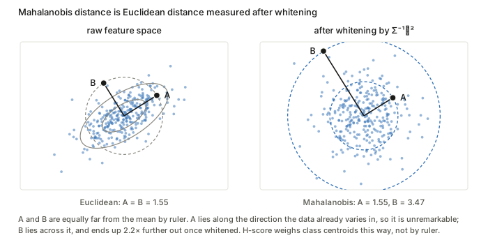
The paper compresses this into one sentence — “a high H-score implies the inter-class variance is large, while feature redundancy is small” — and moves on. The classifier it has in mind is nearest class mean: compute a centroid \mu_y per class and assign x to \arg\min_y\lVert f(x)-\mu_y\rVert. That works exactly when two things hold: the centroids are far apart (or no distance rule can separate them), and the within-class clouds are tight relative to that separation (or points wander into a neighbour’s territory anyway). Those are the numerator and the denominator. \mathcal{H} is the signal-to-noise ratio of a nearest-centroid classifier: centroid separation, measured in units of the feature’s own spread.
That reading is exact, not metaphorical. Expanding \Sigma_B=\sum_y P(y)(\mu_y-\mu)(\mu_y-\mu)^\top and using cyclicity of the trace,
\mathcal{H}(f) = \operatorname{tr}(\Sigma_T^{-1}\Sigma_B) = \sum_y P(y)\,(\mu_y-\mu)^\top\Sigma_T^{-1}(\mu_y-\mu),
so H-score is the average squared Mahalanobis distance from
each class centroid to the global mean. This is what \Sigma_T^{-1} is for: it converts Euclidean
distance into Mahalanobis distance, and a nearest-neighbour rule in the
whitened space is precisely what the score measures. The authors’
function being named getDiffNN suggests this is how they
thought of it.
One consequence of the label entering only through the grouping in step 4: \mathcal{H} is a function of the partition the labels induce, not of the labels themselves. Permuting the class names leaves it unchanged; there is no notion of label ordering or of distance between classes anywhere in it.
Why a denominator with no labels in it measures within-class tightness
The obvious objection to reading \operatorname{cov}(f(X)) as “within-class spread” is that it never sees a label — it is the scatter of all the features about one global mean. The resolution is the law of total covariance:
\underbrace{\operatorname{cov}(f(X))}_{S_T} = \underbrace{\mathbb{E}_Y\big[\operatorname{cov}(f(X)\mid Y)\big]}_{S_W} + \underbrace{\operatorname{cov}\big(\mathbb{E}[f(X)\mid Y]\big)}_{S_B}.
S_T needs no labels to compute, but it still decomposes into a within-class part and a between-class part. So with S_B held fixed — which is exactly what the ratio does — a larger S_T is a larger S_W. The denominator penalises within-class spread without ever being told which class anything belongs to.
That is not just a hand-wave about monotonicity; the ranking is literally identical. Writing \lambda_i for the generalised eigenvalues of (S_B, S_W) — the Fisher ratios — simultaneous diagonalisation gives
\mathcal{H}(f) = \operatorname{tr}(S_T^{-1}S_B) = \sum_i \frac{\lambda_i}{1+\lambda_i},
each term strictly increasing in \lambda_i. Dividing by total scatter and dividing by within-class scatter therefore order features the same way. The label-free form is simply the convenient one to compute, and it bounds the score into [0,\min(k,\lvert\mathcal{Y}\rvert-1)) as a free side effect.
The picture also corrects the “small \operatorname{tr}(\operatorname{cov} f)” reading. What costs you is spread along the direction that separates the classes, not spread as such:
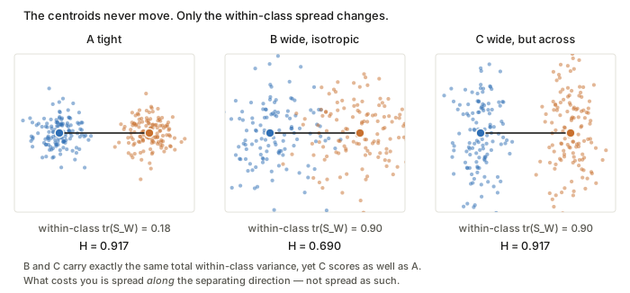
Panels B and C carry identical total within-class variance (\operatorname{tr}(S_W)=0.90) and the centroids never move, yet C scores 0.917 against B’s 0.690 — the same as the far tighter panel A. C’s extra variance is all across the separating direction, where it is free.
What breaks if you drop the denominator
Suppose you scored with \operatorname{tr}(S_B) alone — the plain Euclidean spread of the class centroids. Four things go wrong, in increasing order of seriousness.
- Scale. f\mapsto cf sends \operatorname{tr}(S_B)\mapsto c^2\operatorname{tr}(S_B). Multiplying a feature by 100 multiplies its score by 10{,}000 (0.0123 \to 122.7 in the code) while \mathcal{H} does not move. Since different pre-trained encoders emit wildly different activation scales, and comparing encoders is the entire purpose, this alone disqualifies it.
- Redundancy. Duplicating a feature raises \operatorname{tr}(S_B) (0.00455\to0.00679 in the code) though it adds no new separating direction. You would be rewarded for padding your feature vector with copies.
- The operational meaning evaporates. Theorem 1 derives E_f^k = c\,\mathcal{H}(f) under \operatorname{cov}(f(X))=I. Strip the normalisation and you are no longer computing an error exponent, so the one thing that distinguishes H-score from an arbitrary heuristic is gone.
- It stops being a projection. This is the deepest one. In Eq. 3 the quantity is \lVert\tilde B\Phi(\Phi^\top\Phi)^{-1/2}\rVert_F^2, and (\Phi^\top\Phi)^{-1/2} is precisely what orthonormalises the basis of \Phi. Without it you have \lVert\tilde B\Phi\rVert_F^2, which depends on how you happened to parameterise \Phi rather than on the subspace it spans. The Pythagoras decomposition that made the whole derivation work no longer holds.
Measured, on 40 random features ranked against the true optimal log-loss (Spearman, -1 is perfect), as the per-coordinate scales are spread more widely. Both \mathcal{H} and the log-loss are provably invariant to that rescaling — a linear head absorbs it — so only the \operatorname{tr}(S_B) column can move:
| scale spread | ×1 | ×3 | ×30 |
|---|---|---|---|
| Spearman(\mathcal{H}, log-loss) | −0.965 | −0.965 | −0.965 |
| Spearman(\operatorname{tr}S_B, log-loss) | −0.860 | −0.701 | −0.389 |
What “feature redundancy” actually means
The paper glosses \operatorname{tr}(\operatorname{cov}(f(X))) as “feature redundancy”, which is loose — that trace is total variance, not redundancy. Two things are really going on.
The inverse covariance is a whitening, and it buys invariance: for any invertible A,
\operatorname{tr}\!\big((A\Sigma_TA^\top)^{-1}(A\Sigma_BA^\top)\big) = \operatorname{tr}(\Sigma_T^{-1}\Sigma_B).
So \mathcal{H} measures the feature subspace, not your choice of coordinates, scale or rotation. Without \operatorname{cov}^{-1} you could inflate the score by multiplying f by 10.
Redundancy is then penalised structurally. Because \mathcal{H} is a ratio and depends only on the subspace, a duplicated feature adds no new direction and does not raise the score, where an unnormalised between-class scatter would double-count it. That is the honest version of the paper’s sentence, and it is the mechanism behind the connection to the max-relevance min-redundancy feature-selection literature it cites: the trade-off is automatic rather than hand-designed.
Equivalent forms, and the one worth actually using
Written as \operatorname{tr}(\Sigma_T^{-1}\Sigma_B), Eq. 4 invites you to build two k\times k matrices, invert one, multiply them, and then throw away all but the k diagonal entries. None of that is necessary. Six equivalent expressions, checked against each other to 10^{-14}:
1. It is a Frobenius inner product. For symmetric A,B, \operatorname{tr}(AB)=\sum_i\sum_j A_{ij}B_{ji}=\sum_{ij}A_{ij}B_{ij}, so
\mathcal{H}(f) = \langle \Sigma_T^{-1},\, \Sigma_B\rangle_F = \sum_{ij} (\Sigma_T^{-1})_{ij}(\Sigma_B)_{ij}.
An elementwise multiply and a sum, O(k^2), no matrix product.
2. It is a sum of quadratic forms. \Sigma_B is not generic — it is a sum of \lvert\mathcal{Y}\rvert rank-one terms, \Sigma_B=\sum_y p_y d_yd_y^\top with d_y=\mu_y-\mu. Using \operatorname{tr}(Muv^\top)=v^\top Mu,
\mathcal{H}(f) = \sum_y p_y\, d_y^\top \Sigma_T^{-1} d_y ,
which is \lvert\mathcal{Y}\rvert solves against a vector. This is the Mahalanobis reading above, now as an algorithm.
3. Cholesky, so no inverse is ever formed. With \Sigma_T=LL^\top, d_y^\top\Sigma_T^{-1}d_y=\lVert L^{-1}d_y\rVert^2, so \mathcal{H}=\sum_y p_y\lVert v_y\rVert^2 where Lv_y=d_y by forward substitution. Each class contributes a plain squared Euclidean norm.
4. Flip the trace to the small side. With M\in\mathbb{R}^{\lvert\mathcal{Y}\rvert\times k} holding rows \sqrt{p_y}\,d_y^\top we have \Sigma_B=M^\top M, and cyclicity gives \operatorname{tr}(M\Sigma_T^{-1}M^\top) — a \lvert\mathcal{Y}\rvert\times\lvert\mathcal{Y}\rvert trace. For Taskonomy that is 16\times16 rather than 2048\times2048.
5. No k\times k matrix at all. Take the centred data Z\in\mathbb{R}^{m\times k} and a thin QR, Z=QR. Row i is z_i=R^\top q_i, so d_y=R^\top\bar u_y with \bar u_y the class-y mean of the rows of Q; and since R(R^\top R)^{-1}R^\top=I for square invertible R,
d_y^\top\Sigma_T^{-1}d_y = \bar u_y^\top R\;m(R^\top R)^{-1}\,R^\top\bar u_y = m\lVert\bar u_y\rVert^2 ,
and everything collapses to
\boxed{\;\mathcal{H}(f) = \sum_y \frac{\lVert s_y\rVert^2}{m_y}, \qquad s_y = \sum_{i\,\in\,\text{class } y} q_i \;}
Group-sum the rows of Q by class, take squared norms, divide by class counts. \Sigma_T and \Sigma_B are never built; R is computed and discarded.
6. What it really is: principal angles. Let G\in\mathbb{R}^{m\times\lvert\mathcal{Y}\rvert} be the class-indicator matrix with G_{iy}=1/\sqrt{m_y} when y_i=y; its columns are disjointly supported unit vectors, so G^\top G=I. Then (G^\top Q)_{y\cdot}=s_y^\top/\sqrt{m_y} and
\mathcal{H}(f) = \lVert G^\top Q\rVert_F^2 = \sum_i \cos^2\theta_i ,
where \theta_i are the principal angles between \operatorname{span}(\text{centred features}) and \operatorname{span}(\text{class indicators}) — because the singular values of a product of two orthonormal bases are the cosines of the principal angles between their spans.
This form explains, in one line each, things asserted separately above. Invariance to invertible maps of f: those change the basis of \operatorname{span}(Z), not the subspace. Invariance to permuting class names: permutes the columns of G, not its span. The bound \mathcal{H}<\min(k,\lvert\mathcal{Y}\rvert-1): Z is centred so \mathbf 1\perp\operatorname{span}(Z) while \mathbf 1\in\operatorname{span}(G), forcing one angle to be exactly 90^\circ — the single zero in the measured cosines [0.789,\,0.711,\,0.626,\,0.513,\,0], and the reason \operatorname{rank}(\Sigma_B)=\lvert\mathcal{Y}\rvert-1. And those cosines are the canonical correlations between feature space and label indicators, which closes the loop with the paper’s own remark that \tilde B’s singular values are HGR maximal correlations: H-score is the sum of their squares, arrived at from the other end.
Why form 5 is the one to use
It is not asymptotically cheaper — O(mk^2) dominates either way, exactly as the paper says. The gain is numerical. Forming \Sigma_T=Z^\top Z squares the condition number, whereas QR works at \operatorname{cond}(Z). Against a 128-bit modified-Gram–Schmidt reference, on features made progressively more collinear:
| noise | \operatorname{cond}(Z) | \operatorname{cond}(\Sigma_T) | error, naive \operatorname{tr}(\Sigma_T^{-1}\Sigma_B) | error, QR form |
|---|---|---|---|---|
| 1e−3 | 2.5e3 | 6.3e6 | 2e−10 | 7e−15 |
| 1e−5 | 3.1e5 | 9.7e10 | 2e−06 | 3e−12 |
| 1e−7 | 2.6e7 | 6.5e14 | 5e−03 | 7e−11 |
| 1e−8 | 2.2e8 | 3.5e15 | 6e−03 | 4e−11 |
Three decimal places lost by the textbook expression where the QR form is still exact to ten. That is precisely the near-duplicate hazard documented above, and it is largely an artefact of how the quantity is computed rather than of the quantity itself. At k=2048 on real encoder features I would compute H-score as form 5 and not form 0.
Supplement S2: why H-score is an asymptotic error probability
Consider a binary test on m i.i.d. samples, H_0: x^m\sim P_1 versus H_1: x^m\sim P_2. The Bayesian error decays exponentially, and the rate is the error exponent
E = \lim_{m\to\infty}\min_A -\tfrac1m\log P_e^{(m)}, \qquad\text{i.e.}\qquad P_e^{(m)}\approx 2^{-mE}.
Assume both hypotheses lie in a \chi^2-ball \mathcal{N}_\varepsilon(P_0) and write \phi_i(x)=(P_i(x)-P_0(x))/(\varepsilon\sqrt{P_0(x)}) for their normalised perturbation directions. Then:
- Lemma 1 — the best achievable exponent is E=\frac{\varepsilon^2}{8}\lVert\phi_1-\phi_2\rVert^2+o(\varepsilon^2).
- Lemma 2 — a rule built on a feature statistic \frac1m\sum_i f(x^{(i)}) achieves only E_f=\frac{\varepsilon^2}{8}\langle\xi,\phi_1-\phi_2\rangle^2+o(\varepsilon^2), with \xi(x)=\sqrt{P_0(x)}f(x).
Put those side by side and the picture is immediate:
\text{optimal: } \lVert\phi_1-\phi_2\rVert^2 \qquad\text{vs}\qquad \text{feature } f: \langle\xi,\phi_1-\phi_2\rangle^2 .
The feature gets the squared projection of the discriminative direction onto itself. By Cauchy–Schwarz it is at most the optimum, with equality iff \xi\propto\phi_1-\phi_2. So a feature is useful exactly to the extent that it aligns with the direction separating the classes — a feature orthogonal to it has exponent zero no matter how much variance it carries. Lemma 3 adds the k coordinates up, and Theorem 1 finishes: for whitened features, E_f^k = c\,\mathcal{H}(f) with c independent of f.
Two different asymptotics, and the paper blurs them
- In m. The exponent is defined as a limit. P_e\approx 2^{-mE} is an exponential equality — it means \frac1m\log P_e\to -E, invisible to polynomial prefactors. H-score ranks features by decay rate, not by error at your actual sample size. Two features with equal H-score can behave differently at finite m.
- In \varepsilon. Every lemma carries o(\varepsilon^2). The analysis is a second-order expansion valid when the class-conditionals are close together — which is the opposite of the regime you want.
Reproduced
code/hscore.py works on a small discrete joint, the one
setting where \tilde B can be built,
and checks the chain. The three algebraic steps are exact — no local
assumption is involved in any of them, which is worth knowing, since
only Eq. 1 is approximate:
| check | residual |
|---|---|
| Eq. 2, normal equations \tilde B\Phi=\Psi\Phi^\top\Phi | 3.5e−18 |
| Eq. 3, \lVert\tilde B\rVert^2 - (captured + residual) | 1.4e−17 |
| Eq. 4 vs the projection form of Eq. 3 | 0.0 |
| \lVert\tilde B\rVert_F^2 - \chi^2(P_{XY}\Vert P_XP_Y) | 0.0 |
Eq. 3 really is Eckart–Young: constructing the feature whose \Phi spans the top-k right singular vectors, F = [\sqrt{\mathrm{P}_X}]^{-1}V_k, hits the bound exactly (0.058733 against \sum_{i\le k}\sigma_i^2 = 0.058733), while the best of 300 random rank-3 features reaches only 0.008530 — random subspaces land nowhere near the optimum.
Invariance and redundancy. \mathcal{H}(f)=\mathcal{H}(Af)=\mathcal{H}(100f)=0.005098 for a random invertible A. Adding an exactly duplicated feature moves the raw between-class scatter from 0.004553 to 0.006787 while H-score does not move at all (0.005098, pseudo-inverse) — the duplicate adds no subspace.
The nearest-neighbour identity. The Mahalanobis form above is exact: \operatorname{tr}(S_T^{-1}S_B) and \sum_y P(y)(\mu_y-\mu)^\top S_T^{-1}(\mu_y-\mu) both give 0.0073296924, and permuting the class names returns the same value again — confirming that only the partition matters.
A hazard the paper does not mention. With a near-duplicate and a plain inverse, the picture reverses:
| noise scale | \operatorname{cond}(\operatorname{cov} f) | H |
|---|---|---|
| 1e−2 | 3.5e4 | 0.007988 |
| 1e−4 | 5.0e8 | 0.005993 |
| 1e−7 | 3.2e14 | 0.006018 |
against a true value of 0.005098. As \operatorname{cov}(f(X)) becomes ill-conditioned, the inverse amplifies a direction carrying almost no signal, and the score inflates. At the k=2048 features the paper uses on Taskonomy, with finite samples, this is a live concern and there is no discussion of regularisation or pseudo-inversion anywhere in the paper.
The authors’ own code does reach for
np.linalg.pinv rather than a plain solve — but with
rcond set to 10^{-15},
10^{-10} or 10^{-9} depending on the script. That
tolerance only discards singular values of \operatorname{cov}(f(X)) that are zero to
within machine precision; it does nothing for the near-duplicate regime
in the table above, where the condition number is large (10^4–10^{14}) but no singular value is actually
below the cutoff. So the pseudo-inverse in the reference implementation
is a numerical-stability guard against exact singularity, not a
regulariser against the amplification this table shows — the hazard
survives in the code exactly as it does in the paper’s math.
Does the local assumption bind? Ranking 40 random features by H-score against the log-loss a trained linear head actually reaches (Spearman; -1 is perfect):
| \varepsilon | 0.05 | 0.2 | 0.5 | 1.0 | 2.0 |
|---|---|---|---|---|---|
| \lVert\tilde B\rVert_F^2 | 0.0016 | 0.0297 | 0.2012 | 0.4466 | 0.8371 |
| Spearman | −0.977 | −0.993 | −0.994 | −0.997 | −0.988 |
(These shifted slightly when the log-loss solver was fixed to whiten before descending; the conclusion did not.) I expected this to decay as the dependence grew and it does not — if anything it tightens, because at tiny \varepsilon the log-loss differences between features are themselves tiny and the ranking is resolution-limited. So the local assumption buys the derivation, not the ranking. That is more than the paper claims; it is also a benign setting (random Gaussian features on a random joint), and says nothing about learned features on real data.
Questions and doubts
- Theorem 1 is binary-only. The operational meaning is proved for \lvert\mathcal{Y}\rvert=2. Eq. 4 is then used throughout for multi-class and for 16-way quantised pixel tasks, with the meaning asserted to carry over but never extended. This is the largest gap between what is proved and what is used.
- Fine-tuning voids the guarantee, and the paper says so. “For the operational meaning of transferability to hold exactly, we require the fine tuning layers consist of only linear transformations.” With nonlinear fine-tuning they retreat to relative comparison, which the experiments support but which is an empirical claim.
- No conditioning or regularisation analysis, despite
\operatorname{cov}^{-1} at k=2048. The paper says nothing about it; the
reference implementation does reach for
np.linalg.pinv, withrcondat 10^{-15}, 10^{-10} or 10^{-9} depending on the script (all three verified in the repo). But that only discards singular values which are zero to machine precision, so it guards against exact singularity and not against the near-duplicate amplification in the table above — where the condition number reaches 10^4–10^{14} while no singular value falls below the cutoff. My own numbers bear this out: at noise scales 10^{-2} and 10^{-4} the pseudo-inverse and the plain solve return identical inflated values. So the gap is real in both the paper and the code, and the code’spinvshould not be read as having addressed it. The honest qualifier, from the equivalent forms above: much of this is an artefact of how the score is computed rather than of the score itself. Computing it as a QR of the centred features instead of an inverse of their covariance keeps ten correct digits where the textbook expression has lost three, because it never squares the condition number. The metric is better behaved than the formula the paper writes down. - \lvert\mathcal{X}\rvert finite is assumed throughout and is false for images. It is harmless because \tilde B is eliminated, but it means the derivation never formally covers the setting it is applied to.
- Quantising image outputs to 16 colours is a large intervention justified by one sensitivity figure. How much of the transferability ranking survives the quantisation is not measured against an unquantised baseline, because there isn’t one.
- The empirical validation is ranking correlation, not calibration. Figures 2 and S2 show H-score correlates with log-loss; nothing predicts how much accuracy a transfer will yield. For source selection that is enough, which is the paper’s stated use.
Takeaways
- The chain worth remembering: frozen features \Rightarrow the head is least squares \Rightarrow the loss is Pythagoras \Rightarrow what is left to maximise is a projection. Any time a model’s last layer is linear and the rest is frozen, that decomposition is available, and it converts “how good is this representation?” into “how much of the target structure does this subspace span?”.
- H-score is the Fisher discriminant ratio \operatorname{tr}(S_T^{-1}S_B). The value added is not the statistic but the operational meaning — it is proportional to an error exponent — and the derivation showing it falls out of log-loss rather than being posited.
- The reason it is cheap is structural, not a trick: one forward pass and one k\times k covariance, O(mk^2), versus training a transfer network per source–target pair. The supplement reports under an hour per pair on a CPU workstation at k=2048.
- The invariance to invertible linear maps is the part to internalise. It is why the score is meaningful at all across differently-scaled encoders, and it is what makes “redundancy” a consequence of the geometry rather than a penalty someone added.