Four Fundamental Subspaces
Links
- Interactive version: drag the columns of a 2 × 2 matrix until it goes singular and watch the null space appear; rotate the 3-D least-squares picture while dragging the data points of a line fit; run gradient descent on an underdetermined equation; and drag a test point past a PCA residual-space detector.
- Runnable
code: every number on this page.
make verifyruns it. - Standard references: G. Strang, The Fundamental Theorem of Linear Algebra, American Mathematical Monthly 100(9), 1993, which is where the “four subspaces” picture comes from; and chapters 3–4 of his Introduction to Linear Algebra.
- Related foundations pages: Eckart–Young / low-rank SVD (the best rank-k column space), principal angles (how far apart two column spaces are), and LDA / Fisher discriminant (rank caps on scatter matrices).
- Where these ideas do real work in the paper notes: §9 below has the list. The short version: H-score is a projection onto a column space and its loss is the residual, LogME exists because of what happens when the column space is everything, and the NTK never learns what lies in its null space.
In one paragraph
A matrix A takes an input vector x to an output vector Ax, which is always a combination of A’s columns. Two questions about that map explain most of linear algebra’s “subspace” vocabulary. Which outputs are possible? The set of all possible outputs is the column space. A target outside it cannot be hit exactly, and the best you can do is the closest point inside it. The miss, b-Ax, is the residual, and it always points perpendicular to the column space, into a space of its own: the residual space (formally the left null space N(A^\top)). Which inputs does it not see? The inputs that A sends to zero form the null space. Adding anything from the null space to an input changes nothing about the output, so any equation Ax=b that has a solution has a whole family of them, and a learning rule has to pick one. Gradient descent picks in a very particular way. Row space and column space are the halves that matter; null space and residual space are the halves that get thrown away. Everything else on this page, including least squares, the pseudo-inverse, PCA residual detectors, H-score and the NTK’s frozen component, follows from that split.
1. A matrix times a vector is a combination of its columns
Start with a concrete matrix. Take
A=\begin{bmatrix}1&0\\1&1\\1&2\end{bmatrix},\qquad a_1=\begin{bmatrix}1\\1\\1\end{bmatrix},\quad a_2=\begin{bmatrix}0\\1\\2\end{bmatrix}.
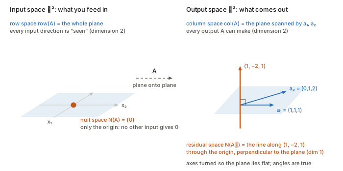
Multiplying by x=(x_1,x_2) does exactly one thing:
Ax = x_1\,a_1 + x_2\,a_2 .
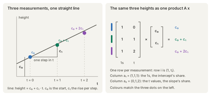
In words: take x_1 times the first column, x_2 times the second, and add. The input x holds the weights and the output is the weighted sum of the columns. This column view is the one to keep in your head, because every subspace below is a statement about which weighted sums are possible and which different weights give the same sum.
This particular A is not arbitrary. It is the design matrix for fitting a straight line y=c_0+c_1t through three points at t=0,1,2. Row i is (1,t_i), so Ax is the list of the line’s heights at the three t values when x=(c_0,c_1) is (intercept, slope). It is the running example for the rest of the page.
| Symbol | Meaning |
|---|---|
| A\in\mathbb R^{m\times n} | the matrix; m outputs (rows), n inputs (columns) |
| r=\operatorname{rank}A | the number of genuinely independent columns |
| \operatorname{col}(A)\subseteq\mathbb R^m | column space: every Ax |
| N(A)\subseteq\mathbb R^n | null space: every x with Ax=0 |
| \operatorname{row}(A)=\operatorname{col}(A^\top)\subseteq\mathbb R^n | row space: every combination of the rows |
| N(A^\top)\subseteq\mathbb R^m | left null space: every y with A^\top y=0; the residual space |
| P=A(A^\top A)^{-1}A^\top | orthogonal projector onto \operatorname{col}(A) (the “hat matrix”) |
| I-P | orthogonal projector onto N(A^\top) (the “residual maker”) |
| A^+ | Moore–Penrose pseudo-inverse |
| V^\perp | orthogonal complement: every vector perpendicular to all of V |
2. Column space: which outputs are possible
Plain words. The column space is the set of every output Ax you can get by choosing some input x. With two columns in \mathbb R^3 it is a plane through the origin: all combinations x_1a_1+x_2a_2 (the shaded plane in Figure 3).
Formally. \operatorname{col}(A)=\{Ax : x\in\mathbb R^n\}=\operatorname{span}(a_1,\dots,a_n). Its dimension is the rank r.
Why it matters. The equation Ax=b has a solution if and only if b lies in the column space. With three data points and a two-parameter line, the heights b=(1,3,2) are not on any straight line (check: the line through the first two points, 1+2t, predicts 5 at t=2, not 2). So b\notin\operatorname{col}(A) and no input x produces it exactly. That is the normal situation in data fitting: more equations than unknowns, so the reachable set is a thin slice of the space the data lives in.
Rank is dimension, not column count. If one column is a mix of the others, it adds no new reachable directions. The rank counts only the independent ones. In the singular example of Figure 1 the matrix has two columns but they point the same way, so the column space is only a line and the rank is 1.
3. Null space: which inputs are invisible
Plain words. The null space is the set of inputs that produce nothing: inputs that A maps to zero. They are the directions of input space that A is blind to.
Formally. N(A)=\{x\in\mathbb R^n : Ax=0\}.
A concrete one. Take the 2\times2 matrix
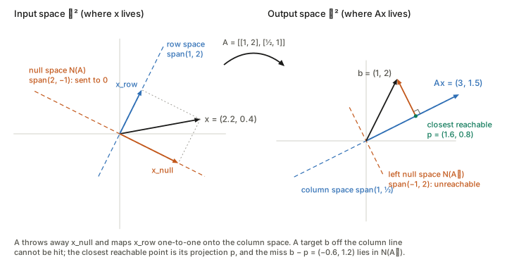
A=\begin{bmatrix}1&2\\ \tfrac12&1\end{bmatrix}.
Its second column is twice the first, so the input x=(2,-1) gives “two of column 1 minus one of column 2” =0. Every multiple of (2,-1) does the same, so N(A)=\operatorname{span}(2,-1), a line through the origin (dashed orange in the left panel of Figure 1).
Two consequences, both important later.
- Solutions come in families. If Ax_0=b and z\in N(A) then A(x_0+z)=b+0=b. Every solution is “one particular solution plus anything from the null space”. When the null space is more than \{0\}, the data alone cannot tell you which solution is right. Something else has to choose: a prior, a penalty or the learning algorithm (§6).
- Information is destroyed. Two inputs that differ by a null-space vector produce the same output, so no procedure can recover the null-space part of x from Ax. A square matrix is invertible exactly when its null space is only \{0\}.
4. The other two, and why they come in perpendicular pairs
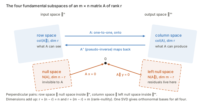
Every matrix has two more subspaces, obtained by asking the same two questions about A^\top:
- Row space \operatorname{row}(A)=\operatorname{col}(A^\top)\subseteq\mathbb R^n: all combinations of the rows. It lives in the input space, next to the null space.
- Left null space N(A^\top)=\{y : A^\top y=0\}\subseteq\mathbb R^m: all vectors perpendicular to every column. It lives in the output space, next to the column space.
Why the pairs are perpendicular. Write out Ax=0 row by row: it says (\text{row}_i)\cdot x=0 for every row. So a null-space vector is perpendicular to every row, and therefore to every combination of rows. That is the whole proof that
\begin{aligned} N(A)&=\operatorname{row}(A)^\perp &&\text{inside }\mathbb R^n,\\ N(A^\top)&=\operatorname{col}(A)^\perp &&\text{inside }\mathbb R^m . \end{aligned}
The second is the same argument applied to A^\top: A^\top y=0 says y is perpendicular to every column. In Figure 1 you can see both right angles: (1,2)\perp(2,-1) on the left and (1,\tfrac12)\perp(-1,2) on the right.
The dimensions add up (the rank–nullity theorem):
\underbrace{r}_{\dim\operatorname{row}}+\underbrace{(n-r)}_{\dim N(A)}=n, \qquad \underbrace{r}_{\dim\operatorname{col}}+\underbrace{(m-r)}_{\dim N(A^\top)}=m .
Row space and column space always have the same dimension r, and A maps one onto the other one-to-one. Everything A does happens between those two; the null space is crushed to zero and the left null space is never reached.
| subspace | lives in | dimension | plain words | in the line fit |
|---|---|---|---|---|
| column space \operatorname{col}(A) | \mathbb R^m (outputs) | r | every output A can make | every straight line’s three heights |
| left null space N(A^\top) | \mathbb R^m | m-r | every possible residual | \operatorname{span}(1,-2,1) |
| row space \operatorname{row}(A) | \mathbb R^n (inputs) | r | the part of the input A uses | all of \mathbb R^2 |
| null space N(A) | \mathbb R^n | n-r | the part of the input A ignores | \{0\}: intercept and slope are identifiable |
The code builds all four from one SVD of a random 5\times4 matrix of rank 2 and confirms the dimensions 2+3=5 and 2+2=4 and both orthogonality relations, to 10^{-16}.
5. Least squares: the residual space is where the misses go
Back to the three points (0,1),(1,3),(2,2). There is no exact line, so least squares asks for the reachable output p=Ax closest to b.
Intuition first. The closest point of a plane to a point off it is the foot of the perpendicular. So the best fit p is the orthogonal projection of b onto the column space, and the miss r=b-p is perpendicular to the plane. Perpendicular to the plane means perpendicular to both columns, and “perpendicular to every column” is precisely the definition of the left null space. Every least-squares residual lives in N(A^\top). That is why this page calls N(A^\top) the residual space.
Now the algebra, which is the same sentence. “r is perpendicular to every column” is A^\top r=0, i.e. A^\top(b-A\hat x)=0, which rearranges to the normal equations
A^\top A\,\hat x = A^\top b .
For the running example, A^\top A=\begin{bmatrix}3&3\\3&5\end{bmatrix} and A^\top b=(6,7), giving
\hat x=\Big(\tfrac32,\ \tfrac12\Big),\qquad p=A\hat x=\Big(\tfrac32,\ 2,\ \tfrac52\Big),\qquad r=b-p=\Big(-\tfrac12,\ 1,\ -\tfrac12\Big)=-\tfrac12\,(1,-2,1).
The fitted line is y=\tfrac32+\tfrac12t, and the three residual bars in the right panel of Figure 3 are -\tfrac12,+1,-\tfrac12: they are the coordinates of r.
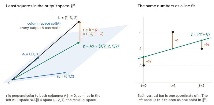
Why the residual always points along (1,-2,1). Here m=3 and r=2, so \dim N(A^\top)=1: the residual space is a single line. Check that (1,-2,1) is on it: a_1\cdot(1,-2,1)=1-2+1=0 and a_2\cdot(1,-2,1)=0-2+2=0. It is the second-difference pattern, which makes sense: any straight line has zero second difference, so this is the one shape of three heights that no line can produce. Whatever three heights you type into widget 2, r comes out as a multiple of it.
Pythagoras. Because p\perp r,
\lVert b\rVert^2=\lVert p\rVert^2+\lVert r\rVert^2:\qquad 14 = 12.5+1.5 .
This is not decoration. It is the identity H-score’s Eq. 3 turns into a transferability score (§9): the total is fixed, so minimising the residual is the same as maximising the captured part.
The two projectors
The map b\mapsto p is a matrix, the hat matrix P=A(A^\top A)^{-1}A^\top (“it puts the hat on b”). The map b\mapsto r is I-P, sometimes called the residual maker. For the running example:
P=\frac16\begin{bmatrix}5&2&-1\\2&2&2\\-1&2&5\end{bmatrix}, \qquad I-P=\frac16\begin{bmatrix}1&-2&1\\-2&4&-2\\1&-2&1\end{bmatrix}=\frac16\,(1,-2,1)(1,-2,1)^\top .
Both are symmetric and idempotent (P^2=P: projecting twice changes nothing), and P(I-P)=0: the two spaces share nothing. Their traces are the dimensions of the spaces they project onto, \operatorname{tr}P=2 and \operatorname{tr}(I-P)=1. The code checks all of it.
Residual degrees of freedom: why you divide by n-p
The trace fact has a statistical meaning worth knowing. If b=Ax_{\text{true}}+\varepsilon with noise \varepsilon\sim\mathcal N(0,\sigma^2I), the residual is r=(I-P)\varepsilon (the signal part is in the column space and is removed exactly). The residual can only use the m-p dimensions of the residual space, so
\mathbb E\lVert r\rVert^2=\sigma^2\operatorname{tr}(I-P)=\sigma^2(m-p).
Dividing by m underestimates the noise, and by more as the model grows, because each column you add removes one more dimension the noise could have used. Dividing by the dimension of the residual space, m-p, is right at every size. LogME’s \beta update is this estimator with p replaced by an effective count \gamma (§9).
Centring is projecting onto a residual space
Fit the simplest model of all, a constant: one column, \mathbf 1=(1,\dots,1). The projection of b is its mean times \mathbf 1, and the residual is b-\bar b\,\mathbf 1: the centred data. The residual space is N(\mathbf 1^\top)=\{v:\sum_iv_i=0\}, every vector whose entries sum to zero, of dimension m-1. So “centre the features” means “project them onto the left null space of the all-ones column”. Widget 2 has a fit a constant switch that shows this in \mathbb R^3: the column space shrinks to the line through (1,1,1) and the residual space grows to the plane perpendicular to it. This one fact produces H-score’s forced right angle in §9.
6. The pseudo-inverse, and which solution gradient descent picks
Least squares handles the case where the column space is too small to contain b. The null space handles the opposite problem: too many solutions. The pseudo-inverse A^+ handles both at once, and Figure 2 shows how. It undoes A on the part where A is one-to-one (column space back to row space) and sends the left null space to zero. So x^+=A^+b is:
- a least-squares solution: it throws away the residual part of b and inverts the rest;
- the minimum-norm one among them: it lives in the row space, with no null-space component, and adding a null-space vector could only make it longer (the two parts are perpendicular, so their squared lengths add).
A concrete underdetermined system. One equation, two unknowns: x_1+2x_2=4. Here A=[1\ \ 2], the row space is \operatorname{span}(1,2), the null space is \operatorname{span}(2,-1), and the solutions form a line parallel to the null space (Figure 4). The minimum-norm solution is the point of that line closest to the origin: x^+=A^+b=(0.8,\,1.6), with norm 1.789.
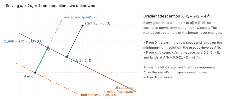
Why gradient descent does this. The gradient of \tfrac12\lVert Ax-b\rVert^2 is A^\top(Ax-b), which is a combination of rows of A, so it always lies in the row space. Every step therefore changes only the row-space part of x. The null-space part is frozen at whatever it was at initialisation:
A start at the origin has no null-space part, so it lands exactly on A^+b. A start elsewhere, such as (3,3) in Figure 4, keeps the null-space part it began with and lands at (2,1).
So gradient descent from zero initialisation returns the minimum-norm solution, and from any other start it returns the minimum-norm solution plus the null-space component it started with. This is the simplest case of what is called the implicit bias of gradient descent: nothing in the loss prefers (0.8,1.6) over (2,1), yet the algorithm reliably picks one. The same statement, for a kernel instead of a row, is the NTK’s “\Delta^0_f never moves” (§9).
7. One SVD gives all four
Write the singular value decomposition A=U\Sigma V^\top with singular values \sigma_1\ge\dots\ge\sigma_r>0 followed by zeros. Then, with no further work:
| subspace | orthonormal basis |
|---|---|
| column space | first r columns of U |
| left null space (residual space) | remaining m-r columns of U |
| row space | first r columns of V |
| null space | remaining n-r columns of V |
The projector onto the column space is U_rU_r^\top and onto the residual space I-U_rU_r^\top, which is the numerically
preferable way to form P (it never
inverts A^\top A, whose condition
number is the square of A’s; the
H-score notes measure that effect). This table is also what the code’s
four_subspaces function does.
Numerical rank needs a threshold. “The number of
nonzero singular values” is not a floating-point question. A matrix
built to have rank 2, plus noise of size 10^{-9}, has singular values 6.8,\ 2.6,\ 2.2\times10^{-9}. NumPy’s default
tolerance calls that rank 3; a tolerance of 10^{-6} calls it rank 2. Which answer is
right depends on whether the 10^{-9}
direction is signal or rounding, and only the user knows.
Pseudo-inverses make the same cut (rcond), which is why
“pinv” in a reference implementation is a statement about what to treat
as null.
Eigenvectors are null spaces too. An eigenvector with eigenvalue \lambda is a nonzero solution of (A-\lambda I)v=0, so an eigenspace is the null space of A-\lambda I. One instance recurs in the contrastive-learning notes: for a graph with normalised adjacency \bar A, the dimension of N(I-\bar A) (the multiplicity of eigenvalue 1) is the number of connected components. The code builds a graph with blocks of 3, 4 and 2 nodes and finds exactly three unit eigenvalues. Add one weak edge between two blocks and the third drops to 0.988, so the null space loses a dimension and a small eigenvalue gap appears in its place.
8. Two things called “residual space”
The phrase is used in two related senses, and papers rarely say which.
- Regression residual space, as above: fix the columns (the regressors), and the residual space is N(A^\top)=\operatorname{col}(A)^\perp, a subspace of the space the targets live in.
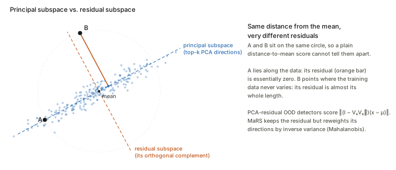
- PCA residual subspace: fit PCA to a cloud of feature vectors, keep the top k principal directions V_k (the principal subspace), and call its orthogonal complement the residual subspace. Each feature splits as x-\mu=V_kV_k^\top(x-\mu)+(I-V_kV_k^\top)(x-\mu), principal part plus residual part.
They are the same idea, “the orthogonal complement of what the model explains”, applied to different objects. In sense 1 the model is a set of regressors and the explained part is the fit. In sense 2 the model is a k-dimensional description of the data and the explained part is the low-rank reconstruction. Eckart–Young says the PCA choice of V_k makes the total residual as small as possible.
Why sense 2 is useful for out-of-distribution detection. Training features typically use only a few directions heavily. A new kind of input can have an ordinary length but point in a direction the training data never used, and that shows up in the residual and nowhere else. In the code, 2,000 training points in \mathbb R^{20} that lie near a 3-dimensional subspace have residual norms with median 0.40 and 99th percentile 0.59. Two test points at the same distance 4.0 from the mean separate completely: one along the data has residual 0.00, one off it has residual 4.00.
9. Where these show up in the other notes
| page | which subspace | what it buys |
|---|---|---|
| H-score, Bao et al. 2019 | column space of the features, and its residual | the score is the captured part of a Pythagoras split; one principal angle is forced to 90^\circ by centring |
| LogME, You et al. 2021 | column space =\mathbb R^n, big null space | why maximum likelihood cannot rank features when D>n, and what “effective degrees of freedom” means |
| LDA and SFDA, Shao et al. 2022 | column spaces of S_b, null space of S_w | the g-1 direction cap; the small-sample singularity and the PCA fix |
| NTK, Jacot et al. 2018 | null space of the kernel | the component the network never learns |
| NTK Selector, Wang et al. 2026 | projection onto a line in matrix space | only the residual of the kernel, its turning, matters |
| Spectral contrastive, HaoChen et al. 2021 and Zhang et al. 2026 | null spaces of Q and of I-\bar A | “up to an invertible map” costs nothing; unit eigenvalues count components |
| Hyperbolic flow matching, Li et al. 2026 | tangent space as a null space | projecting a velocity onto the manifold |
| MICCAI 2026 DA/DG | PCA/Mahalanobis residuals, null space of a forward operator, gradient projection | MaRS, PET-Adapter, PCGrad in MKGA |
| InfoNCE → Gaussian, Betser et al. 2026 | centring as a residual | the cross terms vanish because residuals are perpendicular to the mean |
H-score is least squares, read as a projection. The H-score notes show the frozen-feature head is ordinary least squares (their Eq. 2 is the normal equations), and that the loss splits by Pythagoras (Eq. 3) into a fixed total, a part captured by \operatorname{col}(\Phi) through the projector P=\Phi(\Phi^\top\Phi)^{-1}\Phi^\top, and a residual \tilde B(I-P), “the loss you are stuck with”. That is §5 of this page with \tilde B in place of b. Their form 6 then writes the score as \sum_i\cos^2\theta_i, the principal angles between the column space of the centred features and the span of the class indicators. The bound \mathcal H<\min(k,|\mathcal Y|-1) follows from §5’s centring fact: centring puts \mathbf 1 into the left null space of the features (Z^\top\mathbf 1=0, checked to 10^{-14} in the code), while \mathbf 1 is inside the indicator span (the unnormalised indicator columns add up to it). One direction of the indicator span is therefore perpendicular to the feature span, and one principal angle is exactly 90^\circ. The code’s cosines for four classes are [0.496,\,0.349,\,0.334,\,0.000], with that forced zero last.
LogME exists because the column space can be everything. With D features and n samples, the column space of the n\times D feature matrix is at most n-dimensional. Once D\ge n (and the features are generic), it is all of \mathbb R^n: every label vector is reachable and the least-squares residual is zero. The code gives train R^2=1.000000 for the true features, half-noise features and pure noise alike, each with rank 40 and a 20-dimensional null space of equally perfect weight vectors. That is the LogME table in the notes, explained: maximum likelihood looks only at the residual, and the residual space has vanished. The evidence integrates over the null space instead of picking a point in it. And its noise update \beta^{-1}=\lVert Fm-y\rVert^2/(n-\gamma) is the residual-degrees-of-freedom estimator of §5, with the effective parameter count \gamma in place of p.
LDA and SFDA: rank caps are column-space dimensions. The between-class scatter S_b=\sum_c n_c(\mu_c-\mu)(\mu_c-\mu)^\top is a sum of g rank-one terms whose vectors \mu_c-\mu satisfy one linear relation (their weighted sum is zero), so \dim\operatorname{col}(S_b)\le g-1. Every direction in N(S_b) has zero between-class spread, so the Fisher criterion is zero there. That is why LDA yields at most g-1 directions and why SFDA’s Fisher space is one-dimensional for a binary task. The within-class scatter has rank at most N-g, so when N<n+g it has a nontrivial null space and S_w^{-1} does not exist. A direction in N(S_w) has zero within-class spread, so the Fisher ratio is infinite there. The PCA-then-LDA fix restricts attention to a subspace where S_w has no null space; SFDA’s shrinkage term does the same job by adding a multiple of the identity.
NTK: the null space is never trained. In function space, wide-network training under squared loss is a linear ODE driven by the kernel \Pi, and the error splits over the kernel’s eigenfunctions. The Jacot notes point out that the component \Delta^0_f in the null space of \Pi never moves: directions the kernel cannot see are never learned, at any training time. That is Figure 4 with the kernel playing the role of the row: gradient flow only moves along the directions the operator can see, so the null-space part is fixed by initialisation. The same mechanism leaves an initialisation-dependent term in the trained prediction (it vanishes on the training points, and ensembling cancels it), and it is why overparameterised linear regression trained from zero returns the minimum-norm interpolant.
NTK Selector: a projection in matrix space. The selector notes decompose the evolving kernel as \Theta(t)=a^*(t)\Theta_0+R(t), the least-squares projection onto the line through \Theta_0 plus a residual, using the Frobenius inner product \langle X,Y\rangle=\operatorname{tr}(X^\top Y) on matrices. Perpendicularity gives \lVert R\rVert=\lVert\Theta\rVert\sqrt{1-S^2}, so the cosine S controls the residual. Time reparameterisation then absorbs the projected part exactly, and only the residual survives. The whole argument is §5, with \mathbb R^m replaced by a space of matrices.
Spectral contrastive learning: invertibility means a trivial null space. HaoChen et al.’s Lemma 3.1 says the learned features equal the ideal eigenvector features up to an invertible Q, and that costs a linear probe nothing. Invertible means N(Q)=\{0\}. A rank-deficient Q would have a nonzero null space, and some combination of the eigenvector coordinates would be erased for good. Because only the column space of the feature matrix is pinned down, the notes also observe that individual coordinates are not interpretable; only their span is. And “the multiplicity of eigenvalue 1 counts components” is the N(I-\bar A) fact from §7. Zhang et al. build on the same rank-k factorisation: the minimiser’s column space is the span of the top-k eigenvectors of \bar A.
Hyperbolic flow matching: a tangent space is a null space. On the Lorentz model the manifold is a level set of the Lorentz form \langle z,z\rangle_L=-1/\kappa, and the tangent space at z is every v with \langle z,v\rangle_L=0: the null space of a single row, z^\top J with J=\operatorname{diag}(-1,1,\dots,1). The projection in Li et al., \Pi_{T_zL}(x)=x+\kappa\langle z,x\rangle_L\,z, removes the component of the network’s ambient output along z, the one direction that leaves the manifold; check that \langle z,\Pi_{T_zL}(x)\rangle_L=\langle z,x\rangle_L(1+\kappa\langle z,z\rangle_L)=0. It is an orthogonal projection, but with respect to the Lorentz inner product rather than the Euclidean one (see the caveats).
MICCAI 2026 topic notes: three residual-type constructs. MaRS scores OOD by r^\top\Sigma^{-1}r on the residual of an autoencoder reconstruction, and the topic notes observe that residual-PCA is its hard 0/1 special case: §8’s sense 2, with the residual directions reweighted by their inverse variance. PET-Adapter adapts using only a measurement loss, and the topic notes point out that such a loss cannot constrain the null space of the forward operator A, which is large for limited-angle scans. Whatever fills that null space in the reconstruction comes from the prior, not the data. That is §3’s “information is destroyed” in an imaging costume. PCGrad, used optionally in MKGA, replaces a conflicting gradient g_i by g_i-\frac{g_i^\top g_j}{\lVert g_j\rVert^2}g_j, the residual of regressing g_i on g_j: its projection onto \operatorname{span}(g_j)^\perp.
InfoNCE → Gaussian: centring is a residual. Step 1 of Betser et al.’s bound splits \mathbb E[u\cdot v]=\lVert m\rVert^2+\mathbb E[\tilde u\cdot\tilde v] with \tilde u=u-m. The cross terms, such as \mathbb E[m\cdot\tilde v]=m\cdot\mathbb E[\tilde v], vanish because a mean-zero random vector is orthogonal, in the sense of expectations, to every constant. That is §5’s Pythagoras for the one-column model, used to separate a shared bias from genuine co-variation.
Questions and doubts
- “The residual space” depends on which columns you included. Adding an intercept column shrinks it by one dimension and forces every residual to sum to zero. Centring features before a regression is quietly choosing a model. When a paper reports residual statistics, the column set is part of the definition, and it is often not stated.
- Orthogonal with respect to what? Everything above uses the Euclidean inner product. Weighted least squares projects in the \Sigma^{-1} inner product, Mahalanobis scores measure residuals in it, and the Lorentz projection uses an indefinite form. The four-subspace picture survives, but “perpendicular” and “closest” change meaning, and figures drawn in Euclidean coordinates stop showing the right angles.
- A nonlinear reconstruction has no residual subspace. MaRS’s autoencoder residuals z-D(E(z)) form a set, not a subspace; there is no projector, no guaranteed Pythagoras, and no trace formula for degrees of freedom. The linear picture is the right intuition but not a theorem there.
- The null-space argument for implicit bias is exact only for linear models. For a linearised (NTK-regime) network it holds approximately. Once features move it is at best a heuristic, which is exactly the gap the Fort et al. notes measure.
- Numerical rank is a modelling choice. The tolerance
in
pinvormatrix_rankdecides what counts as null. For ill-conditioned feature matrices (H-score, LogME, SFDA on real backbones), different reasonable tolerances give different null spaces and so different scores.
Takeaways
- A matrix has four subspaces in two perpendicular pairs: row space ⟂ null space in the input space, column space ⟂ left null space in the output space. Their dimensions are r,\ n-r,\ r,\ m-r, and one SVD gives orthonormal bases for all four.
- Column space answers “can this be produced at all?”. Null space answers “what can never be recovered?”. If the null space is nonzero, a solution comes as a family, and something outside the data has to choose among them.
- Least squares is a right angle. The fit is the projection onto the column space. The residual lives in N(A^\top), the residual space, and \lVert b\rVert^2=\lVert p\rVert^2+\lVert r\rVert^2. Its dimension, m-p, is the divisor for the noise variance.
- Centring is projection onto the residual space of the all-ones column. That single fact is why H-score has a forced right angle and why variance estimates lose a degree of freedom.
- Gradient descent never changes the null-space component of its iterate. From zero it finds the minimum-norm solution. That is the NTK’s frozen \Delta^0 and the implicit bias of overparameterised regression.
- “Residual space” means either N(A^\top) for fixed regressors or the complement of a PCA subspace. Both are “the orthogonal complement of what the model explains”, and residual-based OOD detectors score only that part.