Expectation–Maximization (EM) and Gaussian mixtures
Links
- Interactive version: run EM yourself on 2-D clusters one E-step and one M-step at a time (with a k-means switch), step the lower bound of §7 up the log-likelihood, and drag two Gaussians around to see how responsibilities change.
- Source slides: Grosse, Farahmand & Carrasquilla, CSC 411 Lectures 16–17: Expectation-Maximization, University of Toronto. These notes follow the slides’ order but fill in the steps they skip. The derivation in §7–§8 is Bishop, Pattern Recognition and Machine Learning (2006), §9.2–9.4, where the slides’ figures come from.
- LDA / Fisher discriminant: EM with the labels handed to you is exactly fitting the class-conditional Gaussians of LDA (§4). §5 here shows that with shared variances the resulting posterior is a logistic-regression curve.
- Inequalities and concentration: Jensen’s inequality, which is the whole trick in §7.
- Gaussianity in practice: papers that fit Gaussians to CLIP features. A GMM is the natural next step when one Gaussian per class is too crude.
code/em.pychecks every numerical claim below and regenerates the figures:python3 code/em.py --figures.
In one paragraph
You have a cloud of points that looks like it came from a few blobs, and you want to find the blobs. That is a chicken-and-egg problem. If you knew which blob each point came from, fitting each blob would be trivial: take the average and the spread of its points. If you knew the blobs, deciding where each point came from would be trivial too: ask each blob how likely it is to have produced the point. You know neither. EM breaks the loop by guessing one and alternating. Start with rough blobs. E-step: for every point, compute how much each blob is responsible for it (a soft, probabilistic assignment). M-step: refit each blob to the points, weighting each point by that responsibility. Repeat. Each round is guaranteed not to decrease the likelihood of the data, because each round maximises a lower bound that touches the likelihood at the current guess. It converges, though possibly to a local optimum. The same bound is the ELBO that trains VAEs.
1. The chicken-and-egg problem
A concrete version. You measure the heights of 120 people but forgot to write down who is an adult and who is a child. The histogram has two humps. You’d like to report “children average \mu_1 with spread \sigma_1, adults average \mu_2 with spread \sigma_2, and a fraction \pi_1 of the sample are children”.
- If you had the labels, you would split the data and compute two means, two variances and a proportion. Closed form, done (§4).
- If you had the parameters, you could look at one person of height x and ask “how plausible is this height for a child, versus for an adult?”, and get a probability that they are a child (§5).
The label of each point is the missing piece. It is called a latent (hidden) variable, written z: z^{(n)}=k means “point n came from blob k”. EM is the standard way to fit models with a latent variable, and the Gaussian mixture is its standard example.
2. The model: a Gaussian mixture, told as a story
A Gaussian mixture model (GMM) with K components says each data point is produced in two steps:
- Pick a blob. Roll a K-sided die whose faces have probabilities \pi_1,\dots,\pi_K (non-negative, summing to 1). Call the result z. In symbols, z\sim\mathrm{Categorical}(\pi), i.e. p(z=k)=\pi_k.
- Draw from that blob. Sample x from the Gaussian of blob z: x\mid z=k\ \sim\ \mathcal N(\mu_k,\Sigma_k).
The \pi_k are the mixing coefficients, \mu_k the means and \Sigma_k the covariance matrices (in 1-D, just variances \sigma_k^2). All together they are the parameters, written \Theta=\{\pi_k,\mu_k,\Sigma_k\}_{k=1}^K.
The story gives the joint probability of a point and its blob, p(x,z=k)=p(z=k)\,p(x\mid z=k)=\pi_k\,\mathcal N(x\mid\mu_k,\Sigma_k). But we only ever see x. The probability of x alone adds up every way it could have been made (the “sum rule”):
p(x)=\sum_{k=1}^K p(x,z=k)=\sum_{k=1}^K\pi_k\,\mathcal N(x\mid\mu_k,\Sigma_k).
That is a weighted sum of bell curves. In the figure below the two dashed curves are \pi_1\mathcal N(x\mid\mu_1,\sigma_1^2) and \pi_2\mathcal N(x\mid\mu_2,\sigma_2^2), and the solid curve is their sum. One Gaussian fitted to this data would put a single wide hump over the valley in the middle, which is where there’s almost no data. Two Gaussians fit it properly.
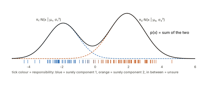
The ticks under the axis are the data, coloured by the E-step answer of §5: blue means “surely blob 1”, orange “surely blob 2”. Points in the valley are a mix. That colouring is the thing EM keeps updating.
Why bother with mixtures? With enough components a GMM can approximate essentially any smooth density (“universal approximator”), even with diagonal covariances. It is also a clustering method with a proper probabilistic score, which lets you compare fits and choose K. That’s what the slides mean by a “generative view of clustering”.
3. Why maximum likelihood is hard here
The usual recipe is to pick \Theta to maximise the log-likelihood of the N data points:
\ell(\Theta)=\ln p(X\mid\Theta)=\sum_{n=1}^N\ln\Big(\sum_{k=1}^K\pi_k\,\mathcal N(x^{(n)}\mid\mu_k,\Sigma_k)\Big).
Read it from the inside out: for each point, add up the K ways it could have been made, take the log, and sum over points. The problem is the sum inside the log. For a single Gaussian, \ln\mathcal N is a simple quadratic in \mu, and setting the derivative to zero gives “\mu = average”. Here the log can’t reach the Gaussians, so every parameter ends up tangled with every other one, and setting derivatives to zero gives no closed form. The slides list three further problems:
- Singularities. Put one component exactly on a
single data point and shrink its variance toward 0. That one point’s
density goes to infinity, and so does the likelihood, while the other
components cover the rest.
em.pydoes this: with the variance at 10^{-4}, 10^{-16}, 10^{-64}, 10^{-256} the log-likelihood goes -339,\,-326,\,-270,\,-49 and keeps climbing. The gain is only \tfrac12\ln(1/\sigma^2), so it’s slow, but it’s unbounded. The “maximum” likelihood is a useless spike. In practice EM sometimes falls into this, and you prevent it by adding a small constant to the diagonal of every \Sigma_k, or by restarting. - Identifiability. Swap the labels “blob 1” and “blob 2” and nothing changes. There are K! equally good answers, so the solution is never unique.
- Non-convexity. There are genuine local optima, not just the relabelled copies. Where you start matters.
4. If we knew the labels: complete data is easy
Suppose someone hands us the true z^{(n)} for every point. Then we don’t need the sum over k because we know which term applies, and the log-likelihood of the complete data (x,z) is
\sum_{n=1}^N\ln p(x^{(n)},z^{(n)}\mid\Theta)=\sum_{n=1}^N\Big[\ln\pi_{z^{(n)}}+\ln\mathcal N\big(x^{(n)}\mid\mu_{z^{(n)}},\Sigma_{z^{(n)}}\big)\Big].
The log now sits directly on each Gaussian. The problem splits into K separate “fit one Gaussian to its own points” problems, each with the familiar answer. Write \mathbb 1[z^{(n)}=k] for “1 if point n is in blob k, else 0” and N_k for the number of points in blob k:
\mu_k=\frac{1}{N_k}\sum_{n}\mathbb 1[z^{(n)}=k]\,x^{(n)},\qquad \Sigma_k=\frac{1}{N_k}\sum_n\mathbb 1[z^{(n)}=k]\,(x^{(n)}-\mu_k)(x^{(n)}-\mu_k)^\top,\qquad \pi_k=\frac{N_k}{N}.
In words: each blob’s mean is the average of its points, its covariance is the spread of its points, and its weight is its share of the data. This is exactly how you fit the class-conditional Gaussians in a Gaussian Bayes classifier or LDA. EM’s M-step (§6) is these same three formulas with the 0/1 indicator replaced by a probability.
5. E-step: responsibilities, from Bayes’ rule
Now go the other way. Fix the parameters and look at one point x. How likely is it that blob k produced it? Bayes’ rule, one line at a time:
\gamma_k(x)\;=\;p(z=k\mid x)\;=\;\frac{p(z=k)\,p(x\mid z=k)}{p(x)}\;=\;\frac{\pi_k\,\mathcal N(x\mid\mu_k,\Sigma_k)}{\sum_{j=1}^K\pi_j\,\mathcal N(x\mid\mu_j,\Sigma_j)}.
The numerator is “how common is blob k” times “how well does blob k explain x”. The denominator is the same thing summed over all blobs, so the \gamma_k for one point add up to 1. \gamma_k^{(n)} is called the responsibility of blob k for point n: a soft vote on where the point came from. If you’ve used a softmax classifier, this is a softmax. The logits are \ln\pi_k+\ln\mathcal N(x\mid\mu_k,\Sigma_k), which for Gaussians is (up to constants) minus half the squared Mahalanobis distance from x to \mu_k.
A worked example. Six points on a line, x=\{1,2,3,6,7,8\}. Start with two blobs, \mu_1=2, \mu_2=4, both variances 1, \pi_1=\pi_2=\tfrac12. The initial guess is bad: blob 2 sits in the gap between the two groups. For x=1 the ratio of the two Gaussian densities is e^{-(1-2)^2/2}/e^{-(1-4)^2/2}=e^{4}\approx55, so \gamma_1=55/56\approx0.982. Doing this for every point:
| x | 1 | 2 | 3 | 6 | 7 | 8 |
|---|---|---|---|---|---|---|
| \gamma_1 (blob at 2) | 0.982 | 0.881 | 0.500 | 0.002 | 0.000 | 0.000 |
| \gamma_2 (blob at 4) | 0.018 | 0.119 | 0.500 | 0.998 | 1.000 | 1.000 |
x=3 is exactly halfway between the two means, so it gets split 50/50. The right-hand group is claimed entirely by blob 2, just because blob 2 is closer to it than blob 1 is.
Two-blob responsibilities are a logistic curve. With equal variances \sigma^2 in 1-D, the ratio of the two numerators is \exp(wx+b) with w=(\mu_1-\mu_2)/\sigma^2 and b=(\mu_2^2-\mu_1^2)/(2\sigma^2)+\ln(\pi_1/\pi_2), so
\gamma_1(x)=\frac{1}{1+e^{-(wx+b)}}.
That’s the logistic-regression sigmoid, the same link between a Gaussian generative model and a linear classifier as in LDA. The third widget of the interactive page plots it. Shrink \sigma and the sigmoid sharpens into a step at the midpoint: that’s k-means (§9).
6. M-step: refit each blob with weighted points
Now treat the responsibilities as fixed and refit. Each blob gets every point, but point n counts only \gamma_k^{(n)} of a point. Take §4’s formulas and replace the indicator \mathbb 1[z^{(n)}=k] by \gamma_k^{(n)}:
N_k=\sum_{n=1}^N\gamma_k^{(n)},\qquad \mu_k=\frac{1}{N_k}\sum_{n}\gamma_k^{(n)}x^{(n)},\qquad \Sigma_k=\frac{1}{N_k}\sum_n\gamma_k^{(n)}(x^{(n)}-\mu_k)(x^{(n)}-\mu_k)^\top,\qquad \pi_k=\frac{N_k}{N}.
N_k is the effective number of points blob k is responsible for. It doesn’t have to be a whole number.
Continuing the example. From the table, N_1=0.982+0.881+0.5+0.002\approx2.37 and N_2\approx3.63. The new means are weighted averages:
\mu_1=\frac{0.982\cdot1+0.881\cdot2+0.5\cdot3+0.002\cdot6}{2.37}\approx1.80,\qquad \mu_2\approx6.26,
with \sigma_1^2\approx0.61, \sigma_2^2\approx3.20, \pi=(0.39,0.61). Blob 2 jumped from the gap to the right-hand group. It is still wide (\sigma_2^2=3.2) because it’s still half-responsible for x=3. The log-likelihood went from -24.3 to -12.7 in one round. After 50 rounds EM settles at the answer you’d pick by eye: \mu=(2,7), \sigma^2=(0.67,0.67), \pi=(\tfrac12,\tfrac12).
The full algorithm (slide 24):
- Initialise \mu_k,\Sigma_k,\pi_k (random data points as means, or the output of k-means).
- E-step: compute \gamma_k^{(n)} for every point and blob with the current parameters.
- M-step: recompute N_k,\mu_k,\Sigma_k,\pi_k from those \gamma’s.
- Compute \ell(\Theta). Stop if it (or the parameters) barely changed, else go to 2.
Here it is on the 120-point data set of §2, starting with two wide, overlapping blobs:
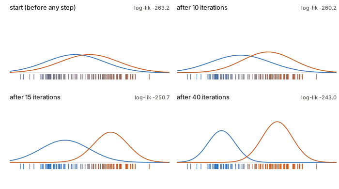
Two things to notice. First, the log-likelihood only ever goes up (−263.2, −260.2, −250.7, −243.0), which §7 explains. Second, for the first ten or so iterations almost nothing happens. The two blobs start nearly symmetric, and a symmetric start is close to a saddle point, where both blobs explain everything equally and neither has a reason to move. EM crawls off such plateaus slowly and then converges quickly. You’ll see the same stall in the interactive page if you start the blobs on top of each other. It’s why k-means initialisation helps.
7. Why it works: a lower bound that touches
The recipe above was motivated by intuition. This section shows it’s actually maximising the likelihood. The whole argument uses one inequality.
Jensen’s inequality for log. \ln bends downward (it’s concave). So if you average some numbers and then take the log, you get at least as much as if you take the logs first and then average:
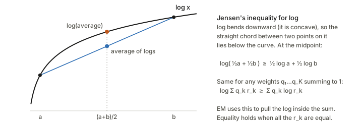
With weights q_1,\dots,q_K\ge0 summing to 1 and any positive numbers r_1,\dots,r_K:
\ln\Big(\sum_k q_k\,r_k\Big)\ \ge\ \sum_k q_k\ln r_k,
with equality exactly when all the r_k are equal (then the “average” is that common value, and the log of it is the same whichever order you do things).
The trick. Our difficulty was the log of a sum, \ln\sum_k p(x,z=k). Take any distribution q(k) over the blobs, for one data point. Multiply and divide by it (this changes nothing):
\ln p(x\mid\Theta)=\ln\sum_k p(x,z=k\mid\Theta)=\ln\sum_k q(k)\,\frac{p(x,z=k\mid\Theta)}{q(k)}.
The right-hand side is now “log of an average of the numbers r_k=p(x,z=k)/q(k), weighted by q”. Jensen lets us swap the log and the average:
\ln p(x\mid\Theta)\ \ge\ \sum_k q(k)\,\ln\frac{p(x,z=k\mid\Theta)}{q(k)}\ =:\ \mathcal L(q,\Theta).
Sum over data points (one q per point) and you get a lower bound \mathcal L on the log-likelihood. The log now sits on p(x,z) directly, just as in the easy complete-data case of §4.
Which q makes the bound tight? Equality needs all the r_k to be equal. Choose q to be the posterior at the current parameters, q(k)=p(z=k\mid x,\Theta^{\text{old}}). Then
r_k=\frac{p(x,z=k\mid\Theta^{\text{old}})}{p(z=k\mid x,\Theta^{\text{old}})}=p(x\mid\Theta^{\text{old}})\quad\text{for every }k,
which is the same number for every k (it’s just Bayes’ rule rearranged). So the bound touches the log-likelihood exactly at \Theta^{\text{old}}. That posterior is the responsibility \gamma_k from §5. The E-step is choosing the q that makes the bound tight.
The M-step then maximises the bound over \Theta with q held fixed. Chaining the three facts:
\ell(\Theta^{\text{old}})\ \overset{\text{tight}}{=}\ \mathcal L(q,\Theta^{\text{old}})\ \overset{\text{M-step}}{\le}\ \mathcal L(q,\Theta^{\text{new}})\ \overset{\text{Jensen}}{\le}\ \ell(\Theta^{\text{new}}).
So the log-likelihood can’t go down. This is the picture on slide 19, drawn here with real curves from the 120-point data (only \mu_1 is varied so it fits on a 2-D plot):
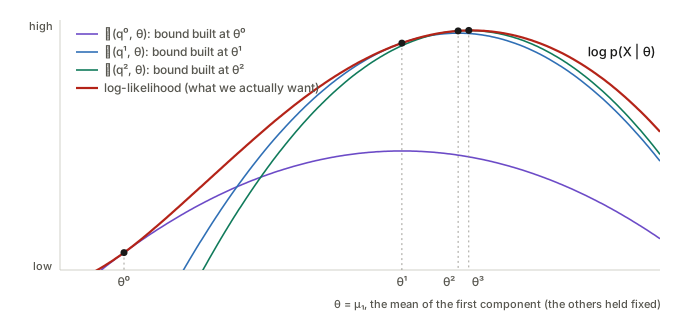
Each coloured curve is the bound built at one iterate. It lies below the red curve everywhere and touches it at that iterate. The next iterate is the top of that bound, which lands higher on the red curve. Repeat. The steps get smaller near the top, which is why EM converges quickly at first and slowly at the end. (The general name for this pattern, “build a touching lower bound, maximise it, repeat”, is minorise–maximise or MM.)
Why is the bound easier to maximise than \ell itself? Expand it:
\mathcal L(q,\Theta)=\underbrace{\sum_n\sum_k\gamma_k^{(n)}\ln p(x^{(n)},z^{(n)}=k\mid\Theta)}_{Q(\Theta,\,\Theta^{\text{old}})}\ \underbrace{-\ \sum_n\sum_k\gamma_k^{(n)}\ln\gamma_k^{(n)}}_{\text{entropy of }q\text{, no }\Theta}.
The second part doesn’t involve \Theta, so the M-step only has to maximise the first part, called the Q-function. For a GMM,
Q=\sum_k\sum_n\gamma_k^{(n)}\ln\pi_k+\sum_k\sum_n\gamma_k^{(n)}\ln\mathcal N(x^{(n)}\mid\mu_k,\Sigma_k),
which splits into K weighted single-Gaussian fits. Solving them (with a Lagrange multiplier for \sum_k\pi_k=1) gives exactly the M-step formulas of §6. The intuitive recipe and the bound argument agree.
8. The same thing as a KL gap
The slides’ “alternative approach” (slides 27–31) says the same thing with one exact identity instead of an inequality. For any distribution q(Z) over the latent variables,
\ln p(X\mid\Theta)=\mathcal L(q,\Theta)+\mathrm{KL}\big(q(Z)\,\Vert\,p(Z\mid X,\Theta)\big).
\mathrm{KL}(q\Vert p)=\sum_Z
q(Z)\ln\frac{q(Z)}{p(Z)} is the Kullback–Leibler
divergence, a measure of how different q is from the true posterior. In plain words,
KL is how badly q guesses where the
points came from. The two facts you need about it: it’s never negative,
and it’s zero only when q equals the
posterior. So the identity says log-likelihood = lower bound +
gap, and the gap is exactly how wrong q is. (em.py checks the identity
numerically for a random q: -289.88 = -363.74 + 73.85.)
Then EM reads as coordinate ascent on \mathcal L:
- E-step: maximise \mathcal L over q with \Theta fixed. The left side doesn’t depend on q, so pushing \mathcal L up means pushing KL down, and the best you can do is \mathrm{KL}=0, i.e. q= posterior. The bound rises to meet the log-likelihood.
- M-step: maximise \mathcal L over \Theta with q fixed. \mathcal L goes up. And now q is stale (it was the posterior for the old \Theta), so a new KL gap opens above it. The log-likelihood goes up by the bound’s increase plus the new gap.
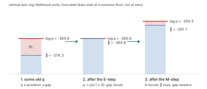
Numbers from em.py for one round: with a stale q, \mathcal
L=-276.3 and a gap of 10.7 under
\ln p=-265.6. The E-step closes the gap
(\mathcal L=-265.6). The M-step raises
\mathcal L to -257.1 and \ln
p to -254.5. That’s a gain of
11.1, more than the 8.5 the bound gained, because a 2.6-sized gap
reopened.
The general algorithm (slide 20), for any latent-variable model, not just GMMs:
- Initialise \Theta^{\text{old}}.
- E-step: compute the posterior p(Z\mid X,\Theta^{\text{old}}), and with it Q(\Theta,\Theta^{\text{old}})=\sum_Z p(Z\mid X,\Theta^{\text{old}})\ln p(X,Z\mid\Theta). The name “expectation” is because Q is the expected complete-data log-likelihood, averaging over the latent variables we can’t see.
- M-step: \Theta^{\text{new}}=\arg\max_\Theta Q(\Theta,\Theta^{\text{old}}).
- Check convergence; else set \Theta^{\text{old}}\leftarrow\Theta^{\text{new}} and go to 2.
The recipe applies whenever the posterior over Z is computable and the complete-data fit is easy: mixtures of other distributions (Bernoulli mixtures for binary data, mixtures of experts), hidden Markov models (the E-step there is the forward–backward algorithm, and the whole thing is Baum–Welch), factor analysis and probabilistic PCA, and missing-data imputation.
9. Relation to k-means
K-means alternates assign (each point to its nearest
centre) and refit (each centre to the mean of its
points). EM alternates soft-assign and weighted
refit. The match is exact in a limit: give every blob the same
covariance \sigma^2 I, fix \pi_k=1/K, and let \sigma\to0. The responsibility softmax has
logits -\lVert
x-\mu_k\rVert^2/(2\sigma^2). As \sigma shrinks, the nearest centre’s logit
dominates all others and \gamma becomes
a one-hot vector. em.py shows it: with \sigma^2=1 only 5% of points have a
responsibility above 0.999, at \sigma^2=0.1 it’s 97%, and at 10^{-3} it’s 99% (the rest sit almost exactly
halfway between centres). The M-step with one-hot weights is the k-means
centre update.
So k-means is “hard EM” for a GMM with round, equal-sized, equally-likely clusters. EM is more flexible: elongated clusters (full \Sigma_k), clusters of different sizes (\pi_k), and an honest “I’m not sure” for points between clusters. The price is more parameters and the singularity of §3. A common practice is to run k-means first and use its clusters to initialise EM.
10. From EM to variational inference (and VAEs)
The E-step needs the exact posterior p(z\mid x,\Theta). For a GMM that’s a K-way softmax. For a model where z is a continuous vector passed through a neural network, there’s no formula. The last slide points at the fix: variational inference. Don’t insist on q= posterior. Pick q from a tractable family, and maximise the same \mathcal L(q,\Theta) over both q and \Theta by gradient ascent. The KL gap no longer closes, so \mathcal L stays a strict lower bound, but it’s still a bound you can climb.
In deep learning this \mathcal L is the evidence lower bound (ELBO), the objective of the variational autoencoder. Rewriting §8’s identity for one data point,
\mathcal L=\mathbb E_{q(z\mid x)}\big[\ln p_\theta(x\mid z)\big]-\mathrm{KL}\big(q(z\mid x)\,\Vert\,p(z)\big).
The first term is the reconstruction term, the second the KL-to-prior term. The encoder network is an amortised q: instead of solving one E-step per data point, it learns to output an approximate posterior for any x in one forward pass. So:
| q (E-step side) | \Theta (M-step side) | |
|---|---|---|
| EM for GMM | exact posterior, in closed form | closed-form weighted fits |
| Variational EM | best member of a tractable family | closed form or gradient step |
| VAE | encoder network q_\phi(z\mid x), gradient step | decoder network p_\theta(x\mid z), gradient step |
11. Practical notes
- Local optima. EM finds a local maximum (or saddle) of \ell, not the global one. Run it from several initialisations and keep the highest log-likelihood.
- Initialisation. K-means centres, or means drawn from the data (k-means++ style), work better than a symmetric start (see the plateau in §6).
- Collapse. Add \epsilon I (say 10^{-6} times the data variance) to every \Sigma_k in the M-step, and restart any blob whose N_k drops near zero.
- Numerics. Compute responsibilities in log space with log-sum-exp. In high dimensions the Gaussian densities underflow to 0 long before anything interesting happens.
- Choosing K. The likelihood always goes up with more components, so compare on held-out log-likelihood or with BIC. (The slides pitch this as a benefit of the probabilistic view: a score to compare clusterings with.)
- Convergence. Stop when the relative change in \ell is below something like 10^{-6}. \ell is non-decreasing, so plotting it is also a good bug check: if your log-likelihood ever goes down, your EM has a bug.
- In scikit-learn:
sklearn.mixture.GaussianMixture(n_components=K, covariance_type="full", n_init=5, reg_covar=1e-6)does all of the above.
Questions and doubts
- Slide 26 says EM for GMMs is soft k-means “with fixed priors and covariance”. That sentence describes the special case that matches k-means (§9). Ordinary GMM EM updates both \pi_k and \Sigma_k.
- Slide 33 says EM converges “maybe to a local minima”. It’s maximising, so the risk is a local maximum (or a saddle point, like the symmetric start in §6).
- Non-decreasing likelihood doesn’t by itself mean the parameters converge. Wu (1983) gives the conditions. For GMMs with the covariance regularised, it’s fine in practice.
Cheat sheet
| Term | One line |
|---|---|
| Latent variable z | the unobserved label, “which blob made this point” |
| Mixture p(x) | \sum_k\pi_k\mathcal N(x\mid\mu_k,\Sigma_k), a weighted sum of bell curves |
| Mixing coefficient \pi_k | prior probability of blob k; non-negative, sums to 1 |
| Complete-data likelihood | p(x,z\mid\Theta). Easy to maximise: the log reaches the Gaussians |
| Responsibility \gamma_k^{(n)} | p(z^{(n)}=k\mid x^{(n)},\Theta) by Bayes’ rule. A softmax over blobs |
| N_k | \sum_n\gamma_k^{(n)}, blob k’s effective number of points |
| E-step | compute the \gamma’s. Equivalently: set q to the posterior, which closes the KL gap |
| M-step | weighted mean, weighted covariance, \pi_k=N_k/N. Equivalently: maximise Q |
| Q(\Theta,\Theta^{\text{old}}) | expected complete-data log-likelihood under the old posterior |
| \mathcal L(q,\Theta) / ELBO | lower bound from Jensen: \ln p(X)-\mathrm{KL}(q\Vert p(Z\mid X)) |
| Guarantee | \ell(\Theta^{\text{new}})\ge\ell(\Theta^{\text{old}}), every iteration |
| k-means | hard EM with shared round covariance \sigma^2I\to0 and equal \pi_k |